In the case of the rod we have the property
\[\bm P_t \mathbf{B} = \mathbf{B}\]Meaning that the derivatives of the basis functions for the rod element are in-line.
Table of contents
In what follows we shall derive the FEM for the rod element using the weak form of the elasticity equation and tangential calculus.
Unlike the direct approach, we will introduce a framework for developing FEM on continuum elements more generally. The resulting linear system will be exactly the same as for the direct approach. However, this approach is more general and applicable to other element types.
A truss system is made of rod elements which only carry loads axially, they still obey the principal of minimum potential energy and the weak form of the elasticity equation.
Consider the following truss system of rods in 2D. We have 3 nodes and 3 elements. The problem states:
Find the displacements of the nodes, \(u\), such that
\[\boxed{ \int_{\Omega } \bm \sigma (\bm u) : \bm \varepsilon \left( \bm v\right) d\Omega =\int_{\Omega } \bm f\cdot \bm vd\Omega +\int_{\partial \Omega } \bm{t} \cdot \bm v ds \quad \forall v \text{ that are } 0 \text{ on } \partial \Omega_D}\]holds under the boundary conditions
\[\left\lbrack u_1^x ,u_1^y ,u_3^x \right\rbrack =0 \text{ and } f_2^y =-P.\]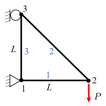
Consider a rod element in 2D
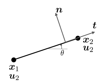
A rod element is defined by having two nodes, connected by a straight line. The nodal displacements are denoted by \(\bm u_1\) and \(\bm u_2\) and correspond to the nodal positions \(\bm x_1\) and \(\bm x_2\). For simplicity we shall define the following in a 2D setting. The element can be arbitrarily oriented in space, we define the angle between the x-axis and the rod as \(\theta\). The tangential vector is given by \(\bm t=\frac{ \bm x_2 -\bm x_1 }{|\bm x_2 -\bm x_1 |}\) and the normal vector is defined as \(\bm n={\bm e }_z \times \bm t\). We note that the tangential vector and the normal vector can be expressed using \(\theta\).
\[\bm t=\left\lbrack \cos \theta ,\sin \theta \right\rbrack\] \[\bm n=\left\lbrack -\sin \theta ,\cos \theta \right\rbrack\]We know from the definition of the element that it only carries axial loads, i.e., in-line loads. Thus the in-line strain has to be
\[ \tilde{\bm \varepsilon} =\left\lbrack \begin{array}{cc} \dfrac{\partial u_x }{\partial x_t } & 0\\ 0 & 0 \end{array}\right\rbrack \]where \( \sim \) denotes the strain tensor in local coordinates. The \(t\) (tangential) subindex in \(\frac{\partial }{\partial x_t }\) denotes that the derivatives are in-line with the element.

In essence, we need to compute the strain tensor such that it has no out of line components, i.e., we need to define an in-line strain tensor, \(\bm \varepsilon_t^P\) such that
\[\bm n\cdot \bm \varepsilon_t^P \cdot \bm n=0\]using this tensor, our weak form takes the form
\[ E\int_{\Omega } \bm \varepsilon_t^P \left(\bm u\right) : \bm \varepsilon_t^P \left(\bm v\right)d\Omega =\int_{\Omega } \bm f\cdot \bm v\;d\;\Omega +\int_{\partial \Omega } \bm t\cdot \bm v ds \quad \forall v=0 \; \textrm{on}\;\partial \Omega \]We need to compute \(\frac{\partial u_x }{\partial x_t }\) numerically.
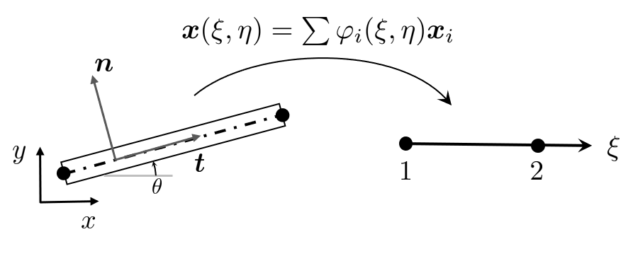
We begin by constructing a parametric map for the rod element. The \(t\) direction of the rod will be mapped to the \(\xi -\)direction and \(n\;\)to \(\eta\) such that any point on the physical rod can be expressed by \(\xi\) and \(\eta\) as such
\[ \bm x (\xi ,\eta ) = \varphi_1 (\xi) \bm x_1 +\varphi_2 (\xi) \bm x_2 + \eta \bm n = \bm x_1 + \xi \left( \bm x_2 - \bm x_1 \right) + \eta \bm n \]where \(\varphi =\left\lbrack 1-\xi ,\xi \right\rbrack\) are the basis functions for the rod element and we let \(\eta \in \left\lbrack -r,r\right\rbrack\) parametrize the thickness of the rod within a radius \(r\) around the centerline.
Now, let the gradient of the displacements
\[ \def\arraystretch{2.5} \nabla \bm u = \left\lbrack \begin{array}{cc} \dfrac{\partial u_x }{\partial x} & \dfrac{\partial u_y }{\partial x}\\ \dfrac{\partial u_x }{\partial y} & \dfrac{\partial u_y }{\partial y} \end{array}\right\rbrack \]We can approximate the derivative using the basis functions, e.g.:
\[\dfrac{\partial u_x }{\partial x}\approx \sum_i \dfrac{\partial \varphi_i }{\partial x}u_i^x =\dfrac{\partial \varphi_1 }{\partial x}u_1^x +\dfrac{\partial \varphi_2 }{\partial x}u_2^x\]which is exact for the rod element, since we assume pure linear deformation.
We can get the derivatives of the basis functions with respect to the spatial variables by the chain rule:
\[ \def\arraystretch{2.5} \left\lbrack \begin{array}{c} \dfrac{\partial \varphi }{\partial \xi }\\ \dfrac{\partial \varphi }{\partial \eta } \end{array}\right\rbrack =\underset{\bm J }{\underbrace{\left\lbrack \begin{array}{cc} \dfrac{\partial x}{\partial \xi } & \dfrac{\partial y}{\partial \xi }\\ \dfrac{\partial x}{\partial \eta } & \dfrac{\partial y}{\partial \eta } \end{array}\right\rbrack } } \left\lbrack \begin{array}{c} \dfrac{\partial \varphi }{\partial x}\\ \dfrac{\partial \varphi }{\partial y} \end{array}\right\rbrack \]where we identify \(\bm J\) as the Jacobian matrix.
\[ \def\arraystretch{2.5} \bm J:=\left\lbrack \begin{array}{cc} \dfrac{\partial x}{\partial \xi } & \dfrac{\partial y}{\partial \xi }\\ \dfrac{\partial x}{\partial \eta } & \dfrac{\partial y}{\partial \eta } \end{array}\right\rbrack \overset{\text{rod element} }{=} \left\lbrack \begin{array}{cc} x_2 -x_1 & y_2 -y_1 \\ n_x & n_y \end{array}\right\rbrack =\left\lbrack \begin{array}{cc} x_2 -x_1 & y_2 -y_1 \\ -\sin \theta & \cos \theta \end{array}\right\rbrack \]The determinant of the Jacobian is a measure of how scaled the size of the physical element is compared to the reference element, i.e., it should be the length, \(L\) for the rod element. Let us check this:
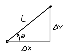
with the geometric relation \(\Delta x=L\;\cos \theta\) and \(\Delta y=L\;\sin \theta\) we have
\[\det \bm J =L\cos^2 \theta +L\sin^2 \theta =L\]Now, the relation (11) can be inverted to get the sought derivatives.
\[ \def\arraystretch{2.5} \left\lbrack \begin{array}{c} \dfrac{\partial \varphi }{\partial x}\\ \dfrac{\partial \varphi }{\partial y} \end{array}\right\rbrack =\bm J^{-1} \left\lbrack \begin{array}{c} \dfrac{\partial \varphi }{\partial \xi }\\ \dfrac{\partial \varphi }{\partial \eta } \end{array}\right\rbrack \]Let
\[ \def\arraystretch{2.5} \hat{\mathbf{B} } :=\left\lbrack \begin{array}{c} \dfrac{\partial \varphi }{\partial \xi }\\ \dfrac{\partial \varphi }{\partial \eta } \end{array}\right\rbrack \overset{\textrm{rod}\;\textrm{element} }{=} \left\lbrack \begin{array}{cc} -1 & 1\\ 0 & 0 \end{array}\right\rbrack \]then
\[ \def\arraystretch{2.5} \left\lbrack \begin{array}{c} \dfrac{\partial \varphi }{\partial x}\\ \dfrac{\partial \varphi }{\partial y} \end{array}\right\rbrack =:\mathbf{B} = \bm J^{-1} \hat{\mathbf{B} } \overset{\textrm{rod}\;\textrm{element} }{=} \dfrac{1}{L}\left\lbrack \begin{array}{cc} -\cos \theta & \cos \theta \\ -\sin \theta & \sin \theta \end{array}\right\rbrack \]We derive this model using the approach by [1] and [2]. Let
\[\mathbf{U}=\left\lbrack \begin{array}{cc} u_1^x & u_1^y \\ u_2^x & u_2^y \end{array}\right\rbrack\]and we can compute the approximate gradient of \(\mathbf U\) by
\[ \def\arraystretch{2.5} \nabla \mathbf U = \mathbf{B} \mathbf U \overset{\textrm{rod}\;\textrm{element} }{=} \left\lbrack \begin{array}{cc} \dfrac{\partial \varphi_1 }{\partial x} & \dfrac{\partial \varphi_2 }{\partial x}\\ \dfrac{\partial \varphi_1 }{\partial y} & \dfrac{\partial \varphi_2 }{\partial y} \end{array}\right\rbrack \left\lbrack \begin{array}{cc} u_1^x & u_1^y \\ u_2^x & u_2^y \end{array}\right\rbrack =\left\lbrack \begin{array}{cc} \dfrac{\partial u_x }{\partial x} & \dfrac{\partial u_y }{\partial x}\\ \dfrac{\partial u_x }{\partial y} & \dfrac{\partial u_y }{\partial y} \end{array}\right\rbrack \]and the typical engineering strain tensor is given by
\[\bm \varepsilon =\dfrac{1}{2}\left(\nabla \bm u^T +\nabla \bm u\right)\]The problem with this tensor is that it is not in-line, i.e., \(\bm n\cdot \bm \varepsilon \cdot \bm n\not= 0\)
We can instead use
\[\bm \varepsilon_t =\dfrac{1}{2}\left(\nabla_t \bm u^T +\nabla_t \bm u\right)\]where
\[\nabla_t \bm u := \bm P_t \nabla \bm u\]and \(\bm P_t\) is known as the tangential projection operator that maps onto the tangent line of the rod. Recall
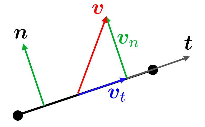
where \(\bm v\) is some out-of-line vector, we can get the in-line vector \(\bm v_t\) by
\[ \bm v_t =\bm v - \bm v_n\]with
\[\bm v_n = \bm n\left(\bm n\cdot \bm v\right)\]Recalling the tensor (outer) product \({\left(\bm a\otimes \mathbf{b}\right)}_{\textrm{ij} } =a_i b_j\) we can use the tensor product rule \(\left(\bm a\otimes \mathbf{b}\right)\bm c=\bm a\left(\mathbf{b}\cdot \bm c\right)\) and get \(\bm v_t =\bm v-\left(\bm n\otimes \bm n\right)\bm v\) which can be rewritten into
\[\bm v_t =\left(\bm I-\bm n\otimes \bm n\right)\bm v=:{\bm P }_t \bm v\]Note that the projection operator also can be written using the tangential vector
\[\bm P_t =\bm t\otimes \bm t\]which has some benefits, since the normal can be hard to define in 3D, especially for the rod.
Using \(\bm t=\left\lbrack \begin{array}{cc} \cos \theta & \sin \theta \end{array}\right\rbrack =\left\lbrack \begin{array}{cc} c & s \end{array}\right\rbrack\) we get the projection operator
\[\bm P_t =\left\lbrack \begin{array}{c} c\\ s \end{array}\right\rbrack \left\lbrack \begin{array}{cc} c & s \end{array}\right\rbrack =\left\lbrack \begin{array}{cc} c^2 & \textrm{cs}\\ \textrm{cs} & s^2 \end{array}\right\rbrack =\left(\bm I-\bm n\otimes \bm n\right)=\left\lbrack \begin{array}{cc} 1 & 0\\ 0 & 1 \end{array}\right\rbrack -\left\lbrack \begin{array}{c} -s\\ c \end{array}\right\rbrack \left\lbrack \begin{array}{cc} -s & c \end{array}\right\rbrack =\left\lbrack \begin{array}{cc} 1-s^2 & \textrm{cs}\\ \textrm{cs} & 1-c^2 \end{array}\right\rbrack\]The problem of using \(\bm \varepsilon_t\) as a measure of strain on the rod is that it is not an in-line tensor, i.e., \(\bm \varepsilon_t \cdot \bm n \not = \bm 0\). Using this tensor we get shear strains associated with the out-of-line direction. To obtain a pure in-line strain tensor we need to apply the projection twice to define
\[\bm \varepsilon_t^P := \bm P_t \bm \varepsilon \bm P_t\]which does not contain any out-of-line strain components, i.e., both the rows and columns of \(\bm \varepsilon_t^P\) are tangent vectors such that \(\bm \varepsilon_t^P \cdot \bm n = \bm n \cdot \bm \varepsilon_t^P = \bm 0 \).
A detailed look at the strain tensor using \(\theta =0\) such that \(\bm n=\left\lbrack 0,1\right\rbrack\) and \(\bm t=\left\lbrack 1,0\right\rbrack\) we get
\[ \def\arraystretch{2.5} \bm P_t =\left\lbrack \begin{array}{cc} 1 & 0\\ 0 & 0 \end{array}\right\rbrack ,\nabla_t \bm u = \bm P_t \nabla u=\left\lbrack \begin{array}{cc} 1 & 0\\ 0 & 0 \end{array}\right\rbrack \left\lbrack \begin{array}{cc} \dfrac{\partial u_x }{\partial x} & \dfrac{\partial u_y }{\partial x}\\ \dfrac{\partial u_x }{\partial y} & \dfrac{\partial u_y }{\partial y} \end{array}\right\rbrack =\left\lbrack \begin{array}{cc} \dfrac{\partial u_x }{\partial x} & \dfrac{\partial u_y }{\partial x}\\ 0 & 0 \end{array}\right\rbrack , \] \[ \def\arraystretch{2.5} \bm \varepsilon_t =\dfrac{1}{2}\left(\left\lbrack \begin{array}{cc} \dfrac{\partial u_x }{\partial x} & 0\\ \dfrac{\partial u_y }{\partial x} & 0 \end{array}\right\rbrack +\left\lbrack \begin{array}{cc} \dfrac{\partial u_x }{\partial x} & \dfrac{\partial u_y }{\partial x}\\ 0 & 0 \end{array}\right\rbrack \right)\left\lbrack \begin{array}{cc} \dfrac{\partial u_x }{\partial x} & \dfrac{1}{2}\dfrac{\partial u_y }{\partial x}\\ \dfrac{1}{2}\dfrac{\partial u_y }{\partial x} & 0 \end{array}\right\rbrack \]and
\[ \def\arraystretch{2.5} \bm \varepsilon_t^P =\left\lbrack \begin{array}{cc} \dfrac{\partial u_x }{\partial x} & 0\\ 0 & 0 \end{array}\right\rbrack \]In the case of the rod we have the property
\[\bm P_t \mathbf{B} = \mathbf{B}\]Meaning that the derivatives of the basis functions for the rod element are in-line.
Recall
\[\mathbf{B}=\dfrac{1}{L}\left\lbrack \begin{array}{cc} -c & c\\ -s & s \end{array}\right\rbrack\]then
\[ \def\arraystretch{1.5} \bm P_t \mathbf B = \left\lbrack \begin{array}{cc} c^2 & c\;s\\ c\;s & s^2 \end{array}\right\rbrack \dfrac{1}{L}\left\lbrack \begin{array}{cc} -c & c\\ -s & s \end{array}\right\rbrack =\dfrac{1}{L}\left\lbrack \begin{array}{cc} -c\left(c^2 +s^2 \right) & c\left(c^2 +s^2 \right)\\ -s\left(c^2 +s^2 \right) & s\left(c^2 +s^2 \right) \end{array}\right\rbrack \]which can also be checked with e.g.,
\[ \def\arraystretch{1.5} \bm P_t \bm t=\left\lbrack \begin{array}{cc} c^2 & c\;s\\ c\;s & s^2 \end{array}\right\rbrack \left\lbrack \begin{array}{c} c\\ s \end{array}\right\rbrack =\left\lbrack \begin{array}{c} c\left(c^2 +s^2 \right)\\ s\left(c^2 +s^2 \right) \end{array}\right\rbrack = \bm t \] \[ \def\arraystretch{1.5} \bm P_t \bm n = \left\lbrack \begin{array}{cc} c^2 & c\;s\\ c\;s & s^2 \end{array}\right\rbrack \left\lbrack \begin{array}{c} -s\\ c \end{array}\right\rbrack =\left\lbrack \begin{array}{c} c^2 s-c^2 s\\ {\textrm{cs} }^2 -{\textrm{cs} }^2 \end{array}\right\rbrack =\left\lbrack \begin{array}{c} 0\\ 0 \end{array}\right\rbrack \]Now that we have an in-line strain tensor we need to implement it into the weak form. We need to compute \(\bm \varepsilon_t^P \left(\bm u\right): \bm \varepsilon_t^P \left(\bm v\right)\) numerically, which can be made easier by working with \(\bm \varepsilon_t\) instead. Using the vector analogy for removing the normal components of the vector, but applied on tensors following the approach by Hansbo and Larson [2], we have for our strain tensor:
\[ \bm \varepsilon_t^P = \bm \varepsilon_t -\left(\bm \varepsilon_t \cdot \bm n\right)\otimes \bm n+\bm n\otimes \left( \bm \varepsilon_t \cdot \bm n\right) \]and the double-dot product
\[ \bm \varepsilon_t^P \left(\bm u \right) : \bm \varepsilon_t^P \left(\bm v \right)= \bm \varepsilon_t \left(\bm u \right) : \bm \varepsilon_t \left( \bm v \right) - 2\left(\bm \varepsilon_t \left(\bm u \right)\cdot \bm n \right) \cdot \left(\bm \varepsilon_t \left(\bm v\right)\cdot \bm n\right) \]Applying Hooke's law for a 1D element, i.e., the in-line stress tensor,
\[ \bm \sigma_t^P = E \bm \varepsilon_t^P \]Thus we arrive at the rod equation, find \(\bm u\) such that
\[E\int_{\Omega } \bm \varepsilon_t \left(\bm u\right): \bm \varepsilon_t \left(\bm v\right)d\Omega -E\int_{\Omega } 2\left(\bm \varepsilon_t \left(\bm u\right)\cdot \bm n\right)\cdot \left(\bm \varepsilon_t \left(\bm v\right)\cdot \bm n\right)d\Omega =\int_{\Omega } \bm f\cdot \bm v\;d\;\Omega +\int_{\partial \Omega } \bm t\cdot \bm v\;\textrm{ds} \quad \forall \bm v=0\;\textrm{on}\;\partial \Omega\]The approximation of the solution vector for the rod element \(K\):
\[ \def\arraystretch{1.5} \begin{array}{l} \bm u_K \left(\bm x \right)\approx {\mathbf U }_K \left(\bm x\right)=\underset{\Phi }{\underbrace{\left\lbrack \begin{array}{cccc} \varphi_1 \left(\bm x\right) & 0 & \varphi_2 \left(\bm x\right) & 0\\ 0 & \varphi_1 \left(\bm x\right) & 0 & \varphi_2 \left(\bm x\right) \end{array}\right\rbrack } } \underset{\mathbf{u} }{\underbrace{\left\lbrack \begin{array}{c} u_1^x \\ u_1^y \\ u_2^x \\ u_2^y \end{array}\right\rbrack } } \\ =\left\lbrack \begin{array}{c} \varphi_1 \left(\bm x\right)u_1^x +\varphi_2 \left(\bm x\right)u_2^x \\ \varphi_1 \left(\bm x\right)u_1^y +\varphi_2 \left(\bm x\right)u_2^y \end{array}\right\rbrack =\left\lbrack \begin{array}{c} U_x \\ U_y \end{array}\right\rbrack =\mathbf U\left(\bm x\right) \end{array} \]The mandel notation for the strain tensor is
\[ \def\arraystretch{2.5} \bm \varepsilon_M \left(\bm u\right)=\left\lbrack \begin{array}{c} \varepsilon_{11} \\ \varepsilon_{22} \\ \sqrt{2}\varepsilon_{12} \end{array}\right\rbrack \approx \left\lbrack \begin{array}{cc} \dfrac{\partial }{\partial x} & 0\\ 0 & \dfrac{\partial }{\partial y}\\ \dfrac{1}{\sqrt{2} }\dfrac{\partial }{\partial y} & \dfrac{1}{\sqrt{2} }\dfrac{\partial }{\partial x} \end{array}\right\rbrack \left\lbrack \begin{array}{c} U_x \\ U_y \end{array}\right\rbrack =\left\lbrack \begin{array}{c} \dfrac{\partial U_x }{\partial x}\\ \dfrac{\partial U_y }{\partial y}\\ \dfrac{1}{\sqrt{2} }\dfrac{\partial U_x }{\partial y}+\dfrac{1}{\sqrt{2} }\dfrac{\partial U_y }{\partial x} \end{array}\right\rbrack \]The double contraction on Mandel form becomes
\[ \bm \varepsilon \left(\bm u\right) : \bm \varepsilon \left(\bm v\right) = \bm \varepsilon_M \left(\bm u\right)\cdot \bm \varepsilon_M \left(\bm v\right) \]thus we have
\[ \bm \varepsilon_t \left(\bm u\right): \bm \varepsilon_t \left(\bm v\right) = \bm \varepsilon_{\textrm{Mt} } \left(\bm u\right)\cdot \bm \varepsilon_{\textrm{Mt} } \left(\bm v\right)={\mathbf{B} }_{\bm \varepsilon }^T {\mathbf{B} }_{\varepsilon } \mathbf{u} \]where
\[ \def\arraystretch{2.5} \mathbf{B}_{\varepsilon } :=\left\lbrack \begin{array}{cccc} \dfrac{\partial \varphi_1 }{\partial x} & 0 & \dfrac{\partial \varphi_2 }{\partial x} & 0\\ 0 & \dfrac{\partial \varphi_1 }{\partial y} & 0 & \dfrac{\partial \varphi_2 }{\partial y}\\ \dfrac{1}{\sqrt{2} }\dfrac{\partial \varphi_1 }{\partial y} & \dfrac{1}{\sqrt{2} }\dfrac{\partial \varphi_1 }{\partial x} & \dfrac{1}{\sqrt{2} }\dfrac{\partial \varphi_2 }{\partial y} & \dfrac{1}{\sqrt{2} }\dfrac{\partial \varphi_2 }{\partial x} \end{array}\right\rbrack \]and for the normal term, we get
\[ \left(\bm \varepsilon_t \left(\bm u\right)\cdot \bm n\right)\cdot \left(\bm \varepsilon_t \left(\bm v\right)\cdot \bm n\right)={\mathbf{B} }_n^T {\mathbf{B} }_n \mathbf{u} \]where
\[ {\mathbf{B} }_n =\left\lbrack \begin{array}{c} n_x \Phi_{1x} +\dfrac{1}{2}n_y \left(\Phi_{1y} +\Phi_{2x} \right)\\ \dfrac{1}{2}n_x \left(\Phi_{1y} +\Phi_{2x} \right)+n_y \Phi_{2y} \end{array}\right\rbrack \]with
\[\begin{array}{l} \Phi_{1x} =\left\lbrack \begin{array}{cccc} \dfrac{\partial \varphi_1 }{\partial x} & 0 & \dfrac{\partial \varphi_2 }{\partial x} & 0 \end{array}\right\rbrack \\ \Phi_{2x} =\left\lbrack \begin{array}{cccc} 0 & \dfrac{\partial \varphi_1 }{\partial x} & 0 & \dfrac{\partial \varphi_2 }{\partial x} \end{array}\right\rbrack \\ \Phi_{1y} =\left\lbrack \begin{array}{cccc} \dfrac{\partial \varphi_1 }{\partial y} & 0 & \dfrac{\partial \varphi_2 }{\partial y} & 0 \end{array}\right\rbrack \\ \Phi_{2y} =\left\lbrack \begin{array}{cccc} 0 & \dfrac{\partial \varphi_1 }{\partial y} & 0 & \dfrac{\partial \varphi_2 }{\partial y} \end{array}\right\rbrack \end{array}\] \[ \int_{\Omega } E\left({\mathbf{B} }_{\varepsilon }^T {\mathbf{B} }_{\varepsilon } -2{\mathbf{B} }_n^T {\mathbf{B} }_n \right)\mathbf{u} d\Omega =\int_{\Omega } E\left({\mathbf{B} }_{\varepsilon }^T {\mathbf{B} }_{\varepsilon } -2{\mathbf{B} }_n^T {\mathbf{B} }_n \right) d\Omega \;\;\mathbf{u} \] \[ \bm S_{e}=\int_{\Omega}E\left(\mathbf{B}_{\varepsilon}^{T}\mathbf{B}_{\varepsilon}-2\mathbf{B}_{n}^{T}\mathbf{B}_{\varepsilon}\right)d\Omega=\int_{-r}^{r}\int_{0}^{1}E\left(\mathbf{B}_{\varepsilon}^{T}\mathbf{B}_{\varepsilon}-2\mathbf{B}_{n}^{T}\mathbf{B}_{\varepsilon}\right)\det\bm{J}d\xi d\eta=EAL\left(\mathbf{B}_{\varepsilon}^{T}\mathbf{B}_{\varepsilon}-2\mathbf{B}_{n}^{T}\mathbf{B}_{\varepsilon}\right) \]As for the right-hand side, we can let \(\bm f = \bm 0\) i.e., no body load and \(\int_{\partial \Omega } \bm t \cdot \bm v ds\) is equivalent to a point load, since the boundary on a rod is just a node. So we treat point loads exactly the same way as in the Systematic Truss Analysis section.
The theory herein serves to unify the 2D elasticity theory with the direct approach and incorporate the rod element into the same framework. The complexity arises when an element of lower dimension is used, as is the case with our rod element which essentially is \(\mathbb R^1\) but embedded into \(\mathbb R^2\) space. That mapping from 1D to 2D is traditionally done using rotational matrices and tricks, which can be omitted using tangential calculus.