Download this page as a Matlab LiveScript

Download StaticElasticity2D.m

Table of contents

2D Static Elasticity Post Processing

(Computing strain and stress from displacements)

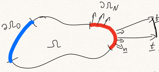
The governing equations of static elasticity for the boundary value problem state:

Problem

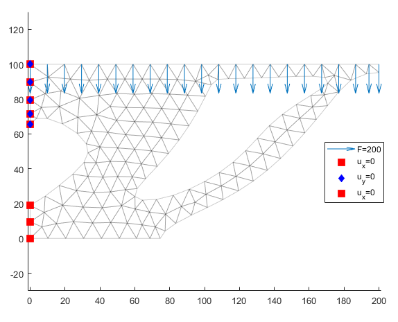
The bracket shown above is designed using topology optimization as inspiration. Topology optimization basically gives us the optimal topology given the constraint that some percentage of material must be removed, in this case 50%. However, topology optimization does not take stress into account, only stiffness. So we need to apply the same loadcase on our optimized bracket and compute the displacements and stresses in order to check if the material can handle the stress.

The material we want to use is a polymer with a elastic modulus of 2200MPa and a Poissons ratio of 0.31. The yield stress is 45MPa. We assume planar stress state and use a thickness of 8mm.

We want to know the following:

• What is the maximum stress? Are there any fictius stress or stress concentration which can be neglected? Where are regions of interest?

• What type of stress is the highest? Pricipal stress or Von Mises?

• We want to know which regions are in tension and which are in compression.

• Is this a good design? Motivate your opinion! Can the design be improved somehow?

• What are your conclusions?

Solution

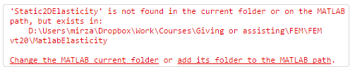
We begin by using Mirzas amazing 2D static elasticity solver in the file Static2DElasticity.m to solve for the displacements. Then we need to compute the strain and stress for each element and at the end we will also do a nodal averaging.

Make sure that the file Static2DElasticity.m is in the current working folder. Otherwise you'll get this error message:

Make sure that you have the PDE Toolbox installed otherwise you'll get errors when running the mesh creation code. (It will work on the school computers)

Geometry

We begin by clearing all variables and load the geometry. Make sure that the STL file is in the current folder. We import the geometry by reading theBracket.stl file.

clear
model = createpde;
importGeometry(model,'Bracket.stl');
pdegplot(model,'EdgeLabels','on')
title('Imported geometry with regions')

From the plot we should be able to see the geometry as well as the region/edge numbers. We will use these numbers to apply boundary conditions and loads.

Mesh

Next we create the mesh from the geometry.

h = 5 %mm

h = 5

mesh = generateMesh(model,'Hmax',h,'Hmin', h/2,...
     'Hgrad',1.99, 'GeometricOrder', 'linear');

Here h sets the element size, Hmax is the maximum size, Hmin the minimum and Hgrad sets how much the size from one element to its neighbor can differ. The parameter GeometricOrder sets if the triangles are linear or quadratic. Note however that this function does not make the midnodes follow the geometry, it just inserts the mid node in the middle of the edge. We still get a more accurate solution but not a higher geometrical accuracy.

The variable mesh is an object that contains certain fields such as mesh.Nodes which contain the coordinates and mesh.Elements which contain the nodal connectivity.

We can easily visualize the mesh by

pdemesh(mesh)

Material parameters and 2D simplification

E = 2200; %MPa
nu = 0.33;
t = 8;%mm

We assume plane stress, meaning we have a thin object

%Plane Stress
lambda = E*nu/(1-nu^2);
mu = E/(2*(1+nu));

The body load is zero, but we still define it.

fload = @(xi,eta)[0;0]; %Body load

Now we use Mirzas solver to create a 2D static elastic model

statElast = Static2DElasticity(mesh, E, nu, lambda, mu, t, fload)

statElast = 
  Static2DElasticity with properties:

     nodes: [933x3 double]
      Area: 9.8808e+03
         P: [558x2 double]
      knod: 3
       neq: 1116
      nele: 933
      nnod: 558
       dim: 2
         E: 2200
        nu: 0.3300
    lambda: 814.7234
        mu: 827.0677
         t: 8
     fload: @(xi,eta)[0;0]
         S: [1116x1116 double]
         F: [1116x1 double]
      mesh: [1x1 FEMesh]
         u: []
     presc: []

statElast.VisualizeMesh;

Note the output from statElast, we are getting a stiffness matrix and a load vector but no displacements, since we did not define the boundary conditions, also, the loadvector is a zero vector since the body load is zero so we need Neumann boundary conditions as well.

Load boundary conditions

We apply the load by using the ComputeSurfaceLoad method of the statElast object. We specify the region, total magnitude of the load and its direction. As a feedback we get a visualization and the applied load vector, the sum of which shuld be the total magnitude.

F1 = statElast.ComputeSurfaceLoad('Region',6, 'Magnitude', 200, 'Direction',[0,-1],'Visualize',1);
F1tot = sum(F1)

F1tot = -200

Dirichlet boundary conditions

Next we need to apply fixtures, which means setting certain degrees of freedom to zero. We do this by using the PrescribeDisplacement method of statElast. Region 4 will be set to 0 displacement in both x and y directions and region 3 we only prescribe to 0 in the x direction. This means that we assume there is a srew at region 4 but no srew at region 3, it just rests at the wall and is free to move in the y-direction.

statElast.PrescribeDisplacement('Region',4,'Ux',0,'Uy',0,'Visualize',1)
statElast.PrescribeDisplacement('Region',3,'Ux',0,'Visualize',1)

Solve the system

u = statElast.Solve;

In order to visualize we need to convert the displacement field to something manageble.

U = [u(1:2:end), u(2:2:end)];

The magnitude of which is

Ur = sqrt(U(:,1).^2+U(:,2).^2);
maxUr = max(Ur)

maxUr = 0.4802

scale = 50;

Let's visualize the displaced bracket

nodes = statElast.nodes;
P = statElast.P;
figure; axis equal;
patch('Faces',nodes,'Vertices',P+U*scale,'FaceColor','interp','CData',Ur,'EdgeAlpha','0.2')
colorbar
title(['Magnitude of the displacements. Scale: ',num2str(scale)])