Table of contents
The stress matrix is given by
Computing the strain
We construct a rectangle under pure tension, meaning we only expect stress in the x-direction.
Material data
E = 2200; %MPa
nu = 0.33;

%Plane Stress
lambda = E*nu/(1-nu^2);
mu = E/(2*(1+nu));

P = [0,0
     3,0
     3,1
     0,1];
U = [0 0
     1 0
     1 0
     0 0]/100;
L = (P(2,1)-P(1,1));epsx = U(2,1) / L;epsy = -nu * epsx;U(3:4,2) = epsy*1;figure
patch(P(:,1),P(:,2),'w')
axis equal tight off; hold on
patch(P(:,1)+U(:,1)*20,P(:,2)+U(:,2)*20,'w','LineStyle',':', ...
'FaceColor','none')
Compute the stress matrix, von Mises stress and principal stresses for the element. Let , . Use plane stress.
Basis functions
phi = @(xi,eta)[(eta-1.0).*(xi-1.0),-xi.*(eta-1.0),eta.*xi,-eta.*(xi-1.0)];
Bh = @(xi,eta)[eta-1, 1-eta, eta, -eta;
               xi-1,  -xi,   xi,  1-xi ];
We shall evaluate the stress in the midpoint.
xi = 0.5; eta = 0.5;J = Bh(xi,eta)*P;
B = J\Bh(xi,eta);Gradient of
gradU = B*U;epsilon = 1/2*(gradU'+gradU)epsilon = 2x2
0.0033 0
0 -0.0011sigma = 2*mu*epsilon + lambda*trace(epsilon)*eye(2)sigma = 2x2
7.3333 0
0 -0.0000Principal stress
[V,D] = eig(sigma);
sigmaPrinc = diag(D);
dir = V;dir = 2x2
1 0
0 1sigmaPrinc = sigmaPrinc(ind)sigmaPrinc = 2x1
7.3333
-0.0000xm = mean(P,1);
hold on; scale = 0.3;
quiver(xm(1),xm(2),dir(1,1),dir(2,1),scale,'b','Displayname','1st principal direction')
quiver(xm(1),xm(2),-dir(1,1),-dir(2,1),scale,'b','HandleVisibility','off')
quiver(xm(1),xm(2),dir(1,2),dir(2,2),scale,'r','Displayname','2nd principal direction')
quiver(xm(1),xm(2),-dir(1,2),-dir(2,2),scale,'r','HandleVisibility','off')
sigma_vm = sqrt(sigma(1,1)^2-sigma(1,1)*sigma(2,2)+sigma(2,2)^2+3*sigma(1,2)^2)sigma_vm = 7.3333annotation(gcf,'textbox',...
[0.030 0.818 0.3 0.14],...
'String', ...
{['$\theta=$',sprintf(' %0.0f',theta),'$^\circ$'], ...
['$\sigma_1=$',sprintf(' %0.2f',sigmaPrinc(1)),'MPa'], ...
['$\sigma_2=$',sprintf(' %0.2f',abs(sigmaPrinc(2))),'MPa'], ...
['$\sigma_{vM}=$',sprintf(' %0.2f',sigma_vm),'MPa']}, ...
'LineStyle','none', ...
'Interpreter','latex', ...
'FitBoxToText','off');
annotation(gcf,'textbox',...
[0.7 0.13 0.130357139504382 0.145238091619242],...
'String', ...
{['$\sigma =\left\lbrack \begin{array}{cc} ',sprintf('%0.2f',sigma(1,1)),' & ',sprintf('%0.2f',sigma(1,2)),' \\ ',sprintf('%0.2f',sigma(2,1)),' & ',sprintf('%0.2f',sigma(2,2)),' \end{array}\right\rbrack$']},...
'LineStyle','none',...
'Interpreter','latex',...
'FitBoxToText','off');
Let's rotate the rectangle 45 degrees and compute the stresses
theta = 45R = [cosd(theta), -sind(theta)
sind(theta), cosd(theta)]R = 2x2
0.7071 -0.7071
0.7071 0.7071P(:,1) = P(:,1)-1.5;
P(:,2) = P(:,2)-0.5;
P = (R*P')';
P(:,1) = P(:,1)+1.5;
P(:,2) = P(:,2)+0.5;
U = (R*U')';
U = U(:,1:2);
P = P(:,1:2);
xi = 0.5; eta = 0.5;
J = Bh(xi,eta)*P;
B = J\Bh(xi,eta);
gradU = B*U;
epsilon = 1/2*(gradU'+gradU)epsilon = 2x2
0.0011 0.0022
0.0022 0.0011sigma = 2*mu*epsilon + lambda*trace(epsilon)*eye(2)sigma = 2x2
3.6667 3.6667
3.6667 3.6667Principal stress
[V,D] = eig(sigma);
sigmaPrinc = diag(D);
dir = V;
dir = 2x2
-0.7071 0.7071
-0.7071 -0.7071We note that the direction dir is parallel to the rotation matrix R.
sigmaPrincsigmaPrinc = 2x1
7.3333
-0.0000sigma_vm = sqrt(sigma(1,1)^2-sigma(1,1)*sigma(2,2)+sigma(2,2)^2+3*sigma(1,2)^2)sigma_vm = 7.3333figure
patch(P(:,1),P(:,2),'w')
axis equal tight off; hold on
patch(P(:,1)+U(:,1)*20,P(:,2)+U(:,2)*20,'w','LineStyle',':', ...
'FaceColor','none')
xm = mean(P,1);
hold on; scale = 0.3;
quiver(xm(1),xm(2),dir(1,1),dir(2,1),scale,'b','Displayname','1st principal direction')
quiver(xm(1),xm(2),-dir(1,1),-dir(2,1),scale,'b','HandleVisibility','off')
quiver(xm(1),xm(2),dir(1,2),dir(2,2),scale,'r','Displayname','2nd principal direction')
quiver(xm(1),xm(2),-dir(1,2),-dir(2,2),scale,'r','HandleVisibility','off')
annotation(gcf,'textbox',...
    [0.030 0.818 0.3 0.14],...
    'String', ...
    {['$\theta=$',sprintf(' %0.0f',theta),'$^\circ$'], ...
    ['$\sigma_1=$',sprintf(' %0.2f',sigmaPrinc(1)),'MPa'], ...
    ['$\sigma_2=$',sprintf(' %0.2f',abs(sigmaPrinc(2))),'MPa'], ...
    ['$\sigma_{vM}=$',sprintf(' %0.2f',sigma_vm),'MPa']}, ...
    'LineStyle','none', ...
    'Interpreter','latex', ...
    'FitBoxToText','off');

annotation(gcf,'textbox',...
    [0.7 0.13 0.130357139504382 0.145238091619242],...
    'String', ...
    {['$\sigma =\left\lbrack \begin{array}{cc} ',sprintf('%0.2f',sigma(1,1)),' & ',sprintf('%0.2f',sigma(1,2)),' \\ ',sprintf('%0.2f',sigma(2,1)),' & ',sprintf('%0.2f',sigma(2,2)),' \end{array}\right\rbrack$']},...
    'LineStyle','none',...
    'Interpreter','latex',...
    'FitBoxToText','off');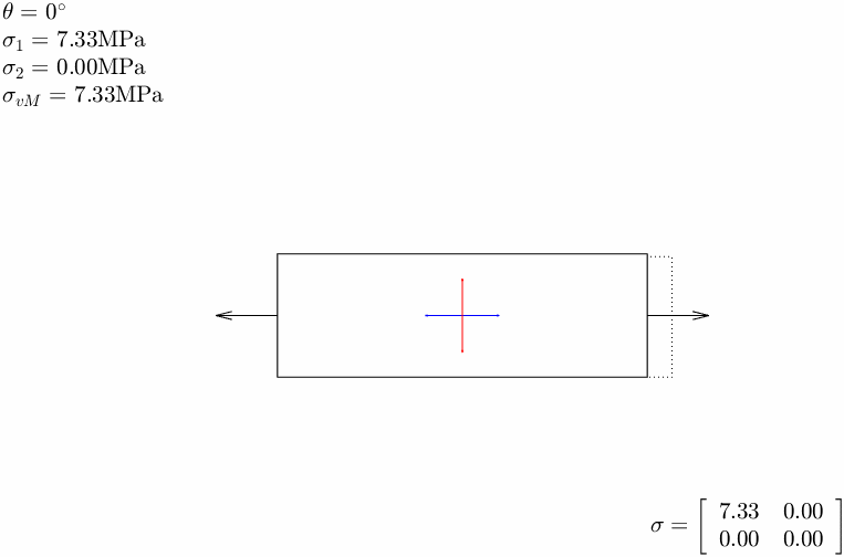
P = [0.1 0.5
0.5 0.8
0.6 0.3];
U = [1 -1
2 -1
0 -2]/50;Compute the stress matrix, von Mises stress and principal stresses for the element. Let , . Use plane stress.
E = 22000; %MPa
nu = 0.3;
lambda = E*nu/(1-nu^2);
mu = E/(2*(1+nu));Basis functions
phi = @(xi,eta)[1-xi-eta, xi, eta];
Bh = @(xi,eta)[-1 1 0
-1 0 1];xi = 1/3; eta = 1/3; % Does not matter for linear elements
J = Bh(xi,eta)*PJ = 2x2
0.4000 0.3000
0.5000 -0.2000B = J\Bh(xi,eta)B = 2x3
-2.1739 0.8696 1.3043
-0.4348 2.1739 -1.7391Gradient of
gradU = B*UgradU = 2x2
-0.0087 -0.0261
0.0783 0.0348epsilon = 1/2*(gradU'+gradU)epsilon = 2x2
0.0031 0.0015
0.0015 0.0009sigma = 2*mu*epsilon + lambda*trace(epsilon)*eye(2)sigma = 2x2
81.8048 24.9527
24.9527 45.3354Principal stresses
[V,D] = eig(sigma);
sigmaPrinc = diag(D);
dir = V;
dir = 2x2
-0.8916 0.4528
-0.4528 -0.8916sigmaPrincsigmaPrinc = 2x1
94.4755
32.6647figure
patch(P(:,1),P(:,2),'w')
axis equal; hold on
patch(P(:,1)+U(:,1),P(:,2)+U(:,2),'w','LineStyle','--', ...
'FaceColor','none')
xm = mean(P,1);
quiver(xm(1),xm(2),dir(1,1),dir(1,2),0.4,'Color','b')
quiver(xm(1),xm(2),dir(2,1),dir(2,2),0.4,'Color','r')

P = [0 0
     1 -0.1
     1.2 1
     -0.1, 1.2];
U = [1 -5
     -1 -5
     -1 5
     1 5]/50;
Let .
Compute the stress matrix in the Gauss points
Compute the von Mises stress in the Gauss points
Compute the von Mises stress in the nodes
Implement Nodal averaging and visualize the von Mises field on the element.
The basis functions for the quadrilateral are given by:
phi = @(xi,eta)[(eta-1.0).*(xi-1.0),-xi.*(eta-1.0),eta.*xi,-eta.*(xi-1.0)];
Bh = @(xi,eta)[eta-1, 1-eta, eta, -eta;
               xi-1,  -xi,   xi,  1-xi ];
Material data
E = 2200; %MPa
nu = 0.33;
%Plane Stress
lambda = E*nu/(1-nu^2);
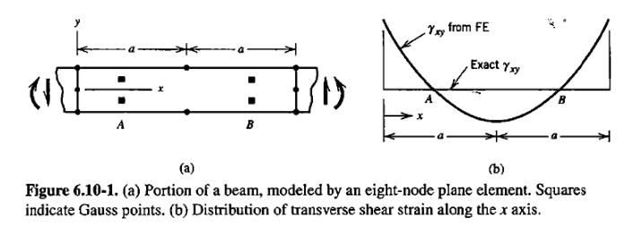
mu = E/(2*(1+nu));Stresses are super convergent at Gauss points, see e.g., Cook Section 6.10 in [1].
Loop over all Gauss points.
figure
patch(P(:,1),P(:,2),'w')
axis equal; hold on
order = 2;
[GP,GW] = GaussQuadrilateral(order);
for ig = 1:4
xi = GP(ig,1);
eta = GP(ig,2);
J = Bh(xi,eta)*P;
B = J\Bh(xi,eta);
gradU = B*U;
epsilon = 1/2*(gradU'+gradU);
sigma = 2*mu*epsilon + lambda*trace(epsilon)*eye(2);
sigma_vm = sqrt(sigma(1,1)^2-sigma(1,1)*sigma(2,2)+sigma(2,2)^2+3*sigma(1,2)^2);
iP = phi(xi,eta)*P;
text(iP(1),iP(2),num2str(sigma_vm))
endLoop over all nodes.
Ph = [0 0
      0 1
      1 1
      1 0];
for ig = 1:4
    xi = Ph(ig,1); eta = Ph(ig,2);

    J = Bh(xi,eta)*P;
    B = J\Bh(xi,eta);
    gradU = B*U;
    epsilon = 1/2*(gradU'+gradU);
    sigma = 2*mu*epsilon + lambda*trace(epsilon)*eye(2);
    sigma_vm = sqrt(sigma(1,1)^2-sigma(1,1)*sigma(2,2)+sigma(2,2)^2+3*sigma(1,2)^2);

    iP = phi(xi,eta)*P;
    text(iP(1),iP(2),num2str(sigma_vm))
end
If we want to take a field that exists inside the element and interpolate it to the nodes, we basically want to minimize
where is the nodal field and the element field. This yields the best average in . The problem states: Find such that
Apply Galerkin and approximate which leads to
or
For our example, using one bi-linear element, we have the von Mises stress in each Gauss point which we want to interpolate to the nodes, so
and
where is the area of the reference element. Thus we can get
Let's implement this in Matlab, loop over all Gauss points
order = 2;
[GP,GW] = GaussQuadrilateral(order);

Me = zeros(4,4);
be = zeros(4,1);
for ig = 1:4
    xi = GP(ig,1); eta = GP(ig,2); iW = GW(ig);

    J = Bh(xi,eta)*P;
    B = J\Bh(xi,eta);
    gradU = B*U;
    epsilon = 1/2*(gradU'+gradU);
    sigma = 2*mu*epsilon + lambda*trace(epsilon)*eye(2);
    sigma_vm = sqrt(sigma(1,1)^2-sigma(1,1)*sigma(2,2)+sigma(2,2)^2+3*sigma(1,2)^2);

    iP = phi(xi,eta)*P;
    Me = Me + phi(xi,eta)'*phi(xi,eta)*det(J)*1*iW;
    be = be + phi(xi,eta)'*sigma_vm*det(J)*1*iW;
end
sigma_vmn = Me\be
sigma_vmn = 4x1
31.3527
35.2472
34.9635
31.9640scale = 1;
figure;
patch(P(:,1)+U(:,1)*scale,P(:,2)+U(:,2)*scale,'w','LineStyle','-', ...
'FaceColor','interp','Cdata',sigma_vmn)
axis equal
colorbar
colormap jet
title('von Mises stress')
We start by creating the geometry using the Partial Differential Toolbox.
clear
R1 = [3,4,0,20,20,0,0,0,8,8]'; %Create a rectangle
C1 = [4,10,5,2,2]'; %Create a circle in the middle with radius 0.3
C1 and R1 need to be concatenated so one of them needs to be increased with zeros.
C1 = [C1;zeros(length(R1)-length(C1),1)];gd holds the geometric description.
gd = [R1,C1];
sf = 'R1-C1'; % Here we remove C1 from R1.
% sf = 'R1'; % Nothing is removed
ns = char('R1','C1')'; % Label the geometric entities, so we know which is which.
g = decsg(gd,sf,ns);
g holds the primitive geometries lines, and arc segments to describe any 2D geometry.
model = createpde;
geometryFromEdges(model,g);

figure
pdegplot(model,'EdgeLabels','on')
axis tight
Solve the static linear elasticity PDE using linear elements.
Let , , the height mm, the width mm, the traction force use plane stress and implement a solver to numerically find the displacement field and compute the nodal averaged von Mises stress field and the nodal averaged principle stress and its directions.
Solution
We start by creating the mesh
h = 1 %mm Overall mesh sizeHere we can use Hedge as a mesh control, in this case we set the mesh size of edge 8,7,5 and 6 to 0.3. The parameter hgrad means how much an element can grow in size from one element to the next.
mesh = generateMesh(model, 'Hmax', h, 'Hmin', h/2,...
    'hgrad',1.5, 'GeometricOrder', 'linear', 'Hedge',{8,0.3,7,0.3,5,0.3,6,0.3});
Next we set the material parameters and thickness of the geometry
E = 210000; %MPa
nu = 0.33;
t = 0.6; %mm

% Plane Stress
lambda = E*nu/(1-nu^2);
mu = E/(2*(1+nu));
The load case is established next
P = mesh.Nodes';
nodes = mesh.Elements';
[nele, knod] = size(nodes);
[nnod, dof] = size(P);
neq = nnod*dof;

H = max(P(:,2))-min(P(:,2))    %mm
traction = [5000/(H*t),0]' % traction load N/mm^2
edge = 1; % The edge on which the load is applied

% Here we compute the traction load and the stiffness matrix
F = TractionLoad(mesh,t,traction,edge);
S = LinElastStiffness(mesh, lambda, mu, t);

% Visualize the mesh
figure; hold on
patch('Vertices', P, 'Faces', nodes,'FaceColor', 'c', ...
    'EdgeAlpha',0.1,'DisplayName','linear mesh')
axis equal tight

% Visualize the load
Finds = findNodes(mesh,'region','Edge',edge);
quiver(P(Finds,1), P(Finds,2), F(Finds*2-1), F(Finds*2-0),'b', ...
    'DisplayName','F=[5000,0]N');

% Apply essential boundary conditions in x-dir
u = zeros(neq,1);
%E1 = findNodes(mesh,'region','Edge',4);
E1 = findNodes(mesh,'nearest',[0;0]) % Get the node at point (0,0)
% Prescribe displacements
u(E1*2) = 0; %y-displacements

% Visualize the boundary conditions in y-dir
plot(P(E1,1),P(E1,2),'bd','MarkerFaceColor','b','Displayname','u_y=0')

% Apply essential boundary conditions in y-dir
E4 = findNodes(mesh,'region','Edge',3);
% prescribed displacement
u(E4*2-1) = 0; %x-displacements

% Visualize the boundary conditions in x-dir
plot(P(E4,1),P(E4,2),'rs','MarkerFaceColor','r','Displayname','u_x=0')

hl = legend('show');
set(hl,'Position',[0.60 0.69 0.20 0.20]);
Apply boundary conditions and solve for the unknown displacement.
presc = unique([E4*2-1, E1*2]);
free = setdiff(1:neq,presc);

F = F - S(:,presc)*u(presc);
u(free) = S(free,free)\F(free);
Visualize the resulting displacement field
U = [u(1:2:end), u(2:2:end)];
UR = sum(U.^2,2).^0.5;
scale = 3;
figure; hold on
pdegplot(model,'EdgeLabels','off')
patch('Vertices', P+U*scale, 'Faces', nodes,'FaceColor', 'interp', ...
    'EdgeAlpha',0.1,'CData',UR)
axis equal tight
title(['Displacement field, scale: ',num2str(scale)])
We verify the displacements first. Use a simple geometry for verification and then change the geometry once the model is verified.
sum(F)                         %N
W = max(P(:,1))-min(P(:,1))    %mm
H = max(P(:,2))-min(P(:,2))    %mm
A = t*H                        %mm^2  Cross sectional area
f = traction(1)*A              %N     Total external load
deltax = f*W/(E*A)             %mm    Total x deformation
epsx = deltax/W                %mm/mm Strain in x-dir
epsy = -nu*(epsx)              %mm/mm Strain in y-dir
deltay = epsy*H                %mm    Total y deformation

sigma_nominal = f/A            %N/mm^2 or MPa stress

ux = max(U(findNodes(mesh,'region','Edge',1),1))
uy = min(U(findNodes(mesh,'region','Edge',2),2))
Without the hole we get:
sum(F) = 5000
W = 20
H = 8
A = 4.0
f = 5000
deltax = 0.0992
epsx = 0.0050
epsy = -0.0016
deltay = -0.0131

sigma_nominal = 1.0417e+03

ux = 0.0992
uy = -0.0131phi = @(xi,eta)[1-xi-eta, xi, eta];
Bh = [-1,1,0
-1,0,1];
GP = [0.5 0
0.5 0.5
0 0.5];
GW = [1/3, 1/3, 1/3];
% Alternative Gauss points
% GP = [1/6 1/6
% 2/3 1/6
% 1/6 2/3];
% GW = 1/3*[1;1;1];
Dir1 = zeros(nele,2);
Dir2 = zeros(nele,2);
sigma_vmE = zeros(nele,1);
Xm = zeros(nele,2);
Sig1 = zeros(nnod,1);
Sig2 = zeros(nnod,1);
M = zeros(nnod,nnod);
b = zeros(nnod,1);
for iel = 1:nele
inod = nodes(iel,:);
iP = P(inod,:);
iU = U(inod,:);
J = Bh*iP;
area = det(J)*1/2;
B = J\Bh;
gradU = B*iU;
epsilon = 1/2*(gradU'+gradU); % Verify these by comparing the epsx and epsy
sigma = 2*mu*epsilon + lambda*trace(epsilon)*eye(2); % Verify by comparing to sigma_nominal
sigma_vm = sqrt(sigma(1,1)^2-sigma(1,1)*sigma(2,2)+sigma(2,2)^2+3*sigma(1,2)^2);
[V,D] = eig(sigma, 'vector');
dir = V;
Dir1(iel,:) = dir(:,1);
Dir2(iel,:) = dir(:,2);
sigmaPrinc= D(ind);
sig1 = sigmaPrinc(1);
sig2 = sigmaPrinc(2);
Xm(iel,:) = mean(iP,1)+mean(iU)*scale;
sigma_vmE(iel) = sigma_vm;
xi = 1/3; eta = 1/3; iw = 1;
b(inod) = b(inod) + phi(xi,eta)'*sigma_vm*area*iw;
Sig1(inod) = Sig1(inod) + phi(xi,eta)'*sig1*area*iw;
Sig2(inod) = Sig2(inod) + phi(xi,eta)'*sig2*area*iw;
Me = zeros(3,3); be = zeros(3,1);
for ig = 1:3
xi = GP(ig,1); eta = GP(ig,2);
iw = GW(ig);
Me = Me + phi(xi,eta)'*phi(xi,eta)*area*iw;
end
M(inod,inod) = M(inod,inod) + Me;
end
sigma_vmn = M\b;
Sig1 = M\Sig1;
Sig2 = M\Sig2;
figure
patch('Faces',nodes,'Vertices',P+U*scale, 'EdgeAlpha', 0.2, ...
'FaceColor','flat','CData',sigma_vmE)
axis equal off; hold on;
title('von Mises stress, element values')
colorbar; colormap jet
caxis([0, max(sigma_vmE)])
max(sigma_vmE)ans = 5.4222e+03figure
patch('Faces',nodes,'Vertices',P+U*scale, 'EdgeAlpha', 0.2, ...
'FaceColor','interp','CData',sigma_vmn)
axis equal off; hold on;
title('von Mises stress, nodal averaged')
colorbar; colormap jet
caxis([0, max(sigma_vmn)])
max(sigma_vmn)ans = 5.3091e+03figure
patch('Faces',nodes,'Vertices',P+U*scale, 'EdgeAlpha', 0.2, ...
'FaceColor','interp','CData',Sig1)
axis equal off; hold on;
title('First principal stress, nodal averaged')
colorbar; colormap jet
quiver(Xm(:,1),Xm(:,2),Dir1(:,1),Dir1(:,2),0.2,'ShowArrowHead','off','Color','k')
caxis([min(Sig1), max(Sig1)])
max(Sig1)ans = 5.5595e+03min(Sig1)ans = -1.6973e+03function F = TractionLoad(mesh,t,fload,edge)
P = mesh.Nodes';
nodes = mesh.Elements';
[nele, knod] = size(nodes);
[nnod, dof] = size(P);
neq = nnod*dof;
phi=@(xi)[1-xi,xi];
Einds = findNodes(mesh,'region','Edge',edge);
eleInds = find(sum(ismember(nodes,Einds),2)>1);
F = zeros(neq,1);
ieqs = zeros(2*2,1);
PHI = zeros(2,4);
L = 0;
nele = length(eleInds);
for iel = 1:nele
indTri = eleInds(iel);
iTri = nodes(indTri,:);
iEdgeNodes = iTri(ismember(iTri,Einds));
ieqs(1:2:end) = 2*iEdgeNodes-1; %x-dofs
ieqs(2:2:end) = 2*iEdgeNodes-0; %y-dofs
xc = P(iEdgeNodes,:);
h = norm(xc(end,:)-xc(1,:));
L = L + h;
xi = 0.5; iw = 1;
PHI(1,1:2:end) = phi(xi);
PHI(2,2:2:end) = phi(xi);
fe = PHI'*fload(:)*t*h*iw;
F(ieqs) = F(ieqs) + fe;
end
endfunction S = LinElastStiffness(mesh, lambda, mu, t)
P = mesh.Nodes';
nodes = mesh.Elements';
[nele, knod] = size(nodes);
[nnod, dof] = size(P);
neq = nnod*dof;
phi = @(xi,eta)[1-xi-eta, xi, eta];
Bh = [-1,1,0
-1,0,1];
S = zeros(neq,neq);
sq = 1/sqrt(2);
for iel = 1:nele
inod = nodes(iel,:);
iP = P(inod,:);
locdof = zeros(1,6);
locdof(1:2:end) = inod*2-1;
locdof(2:2:end) = inod*2;
J = Bh*iP;
area = det(J) * 1/2;
B = J\Bh;
Beps = zeros(3,6);
Beps(1,1:2:end) = B(1,:);
Beps(2,2:2:end) = B(2,:);
Beps(3,1:2:end) = sq*B(2,:);
Beps(3,2:2:end) = sq*B(1,:);
Bdiv = zeros(1,6);
Bdiv(1:2:end) = B(1,:);
Bdiv(2:2:end) = B(2,:);
Se = t*(2*mu*Beps'*Beps + lambda*Bdiv'*Bdiv)*area;
S(locdof, locdof) = S(locdof, locdof) + Se;
end
endfunction [GP,GW] = GaussQuadrilateral(order)
%GaussQuadrilateral Gauss integration scheme for quadrilateral 2D element
% [x,y] in [0,1]
[gp,gw] = gauss(order,0,1);
[GPx,GPy] = meshgrid(gp,gp);
[Gw1,Gw2] = meshgrid(gw,gw);
GW = [Gw1(:), Gw2(:)];
GW = prod(GW,2);
GP = [GPx(:), GPy(:)];
end
function [x, w, A] = gauss(n, a, b)
%------------------------------------------------------------------------------
% gauss.m
%------------------------------------------------------------------------------
%
% Purpose:
%
% Generates abscissas and weights on I = [ a, b ] (for Gaussian quadrature).
%
%
% Syntax:
%
% [x, w, A] = gauss(n, a, b);
%
%
% Input:
%
% n integer Number of quadrature points.
% a real Left endpoint of interval.
% b real Right endpoint of interval.
%
%
% Output:
%
% x real Quadrature points.
% w real Weigths.
% A real Area of domain.
%------------------------------------------------------------------------------
% 3-term recurrence coefficients:
n = 1:(n - 1);
beta = 1 ./ sqrt(4 - 1 ./ (n .* n));
% Jacobi matrix:
J = diag(beta, 1) + diag(beta, -1);
% Eigenvalue decomposition:
%
% e-values are used for abscissas, whereas e-vectors determine weights.
%
[V, D] = eig(J);
x = diag(D);
% Size of domain:
A = b - a;
% Change of interval:
%
% Initally we have I0 = [ -1, 1 ]; now one gets I = [ a, b ] instead.
%
% The abscissas are Legendre points.
%
if ~(a == -1 && b == 1)
x = 0.5 * A * x + 0.5 * (b + a);
end
% Weigths:
w = V(1, :) .* V(1, :);
end