NumericalIntegration

Download this page as a Matlab LiveScript

Table of contents

Video lectures
Integration rules
Numerical integration
Trapezoidal rule
Exact numerical integration
Gauss quadrature rule
Non trivial integrals
1. Example - A tricky integral
2. Example - A sinusoidal
Gauss visualized
Deriving the Gaussian quadrature rule
1. Solving non-linear system of equations
Code snippets

Integration rules

We want to integrate some function $f\left(x\right)$

\int_a^b f\left(x\right)\;d\;x\;

We can take any range $x\in \left\lbrack a,\;b\right\rbrack$ and map it to the range $\xi \in \left\lbrack 0,1\right\rbrack$ using iso-parametric mapping:

$x\left(\xi \right):=\left(1-\xi \right)a+\xi b$ and its derivative (or map) $\frac{d\;x}{d\;\xi }=b-a$ then we have

\int_a^b f\left(x\right)\;d\;x\;=\int_0^1 f\left(x\left(\xi \right)\right)\;\dfrac{d\;x}{d\;\xi }\;d\xi =\left(b-a\right)\int_0^1 f\left(x\left(\xi \right)\right)\;d\;\xi

Let's say we want to integrate some polynomial of order $n$

\int_a^b x^n \;d\;x\;=\left(b-a\right)\int_0^1 {x\left(\xi \right)}^n \;d\;\xi =\left(b-a\right)\int_0^1 {\left(\left(1-\xi \right)a+\xi b\right)}^n d\xi =-\dfrac{a^{n+1} -b^{n+1} }{n+1}

Ok, so this can be used to integrate e.g.,

\int_2^5 2x-4x^2 \;d\;x=-2\dfrac{a^{1+1} -b^{1+1} }{1+1}--4\dfrac{a^{2+1} -b^{2+1} }{2+1}=-135

But in general it is awkward to use this rule to integrate e.g.,

$\int_{x_1 }^{x_2 } \left(1-x\right)\left(1-x\right)\;d\;x$ or $\int_{x_1 }^{x_2 } {\varphi }^T \varphi \;d\;x$ without additional preparation which makes it cumbersome to implement in a computer program and run efficiently.

The same goes for the integration rulse such as

\int_{-1}^1 x^n \;d\;x=\left\lbrace \begin{array}{ll} \dfrac{2}{n+1} & \textrm{if}\;n\;\textrm{is}\;\textrm{even}\\ 0 & \textrm{if}\;n\;\textrm{is}\;\textrm{odd} \end{array}\right.

and

\int_0^1 x^n \;d\;x=\dfrac{1}{n+1}

Numerical integration

Let's consider a polynomial function $f\left(x\right)=1+3x^2 -x^3$ for $x\in \left\lbrack 0,3\right\rbrack$

clear
f = @(x) 1+3*x.^2-x.^3;
a = 0; b = 3;
figure
fplot(f,[a,b])
axis([a,b,0,5.1]); box off;
legend('show','Location','Northwest');

We can integrate this analytically

I_e = int(f,sym("x"),a,b)

\frac{39}{4}

I_e = double(I_e)

I_e = 9.7500

We can also use the numerical integration using the build in variable precision arithmatic integration

vpaintegral(f,sym("x"),a,b)

9.75

This uses a numerical method for integration, is powerful and easy to use, drawback are a default high number of function evaluations.

Now, let's go back to basics and take a look at the Riemann sum.

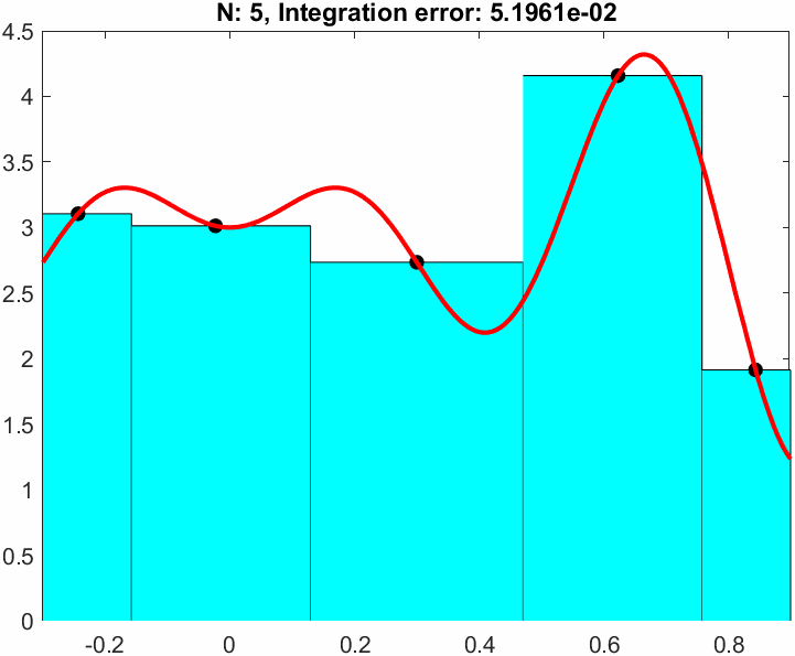
\int_a^b f\left(x\right)\approx \dfrac{b-a}{N}\sum_{i=1}^N f\left(x_i \right)

N = 5;
xnod = linspace(a,b,N);
y = double(f(xnod));
figure
fplot(f,[a,b])
axis([a,b,0,5.1]); box off;
legend('show','Location','Northwest');hold on
hb = bar(xnod,y,1,'LineStyle','-',DisplayName="Riemann Sum");
dx = (b-a)/N;
I_R = sum(y*dx);
ht = title(['$I\approx$ ', sprintf('%0.2f', I_R),', $I = $', sprintf(' %0.2f', I_e),', $N=$ ',sprintf(' %d', N)]);
ht.Interpreter = "latex";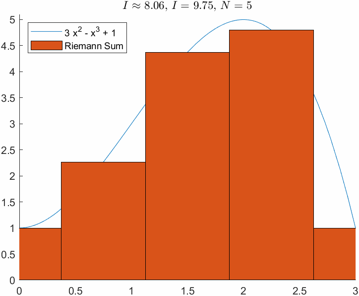

Let's take a look at the error we're making numerically

\epsilon ={\left|I\right.}_{\textrm{Riemann} } -I_{\textrm{exact} } \left|\right.

N = 200;
xnod = linspace(a,b,N);
dx = (b-a)/N;
I_R = sum(f(xnod)*dx);
err_R = abs(I_R-I_e)

err_R = 0.0339

Note that the absolute integration error is still significantly large after 200 function evaluations!

Trapezoidal rule

We can do a better numerical approximation

First we approximate $f\left(x\right)\;$ linearly: $f\left(x\right)\approx \varphi_1 \left(x\right)f\left(a\right)+\varphi_2 \left(x\right)f\left(b\right)=\frac{b-x}{b-a}f\left(a\right)+\frac{x-a}{b-a}f\left(b\right)$ then we have

I\approx \dfrac{f\left(a\right)}{b-a}\int_a^b b-x\;d\;x+\dfrac{f\left(b\right)}{b-a}\int_a^b x-a\;d\;x=\dfrac{f\left(a\right)}{b-a}{\left\lbrack b\;x-\dfrac{1}{2}x^2 \right\rbrack }_a^b +\dfrac{f\left(b\right)}{b-a}{\left\lbrack \dfrac{1}{2}x^2 -a\;x\right\rbrack }_a^b

=\dfrac{f\left(a\right)}{b-a}\left(b^2 -\dfrac{1}{2}b^2 -a\;b-\dfrac{1}{2}a^2 \right)+\dfrac{f\left(b\right)}{b-a}\left(\dfrac{1}{2}b^2 -a\;b-\dfrac{1}{2}a^2 -a^2 \right)

=\dfrac{f\left(a\right)}{b-a}\dfrac{1}{2}{\left(b-a\right)}^2 +\dfrac{f\left(b\right)}{b-a}\dfrac{1}{2}{\left(b-a\right)}^2

=\dfrac{1}{2}\left(b-a\right)\left(f\left(a\right)+f\left(b\right)\right)

This is called the trapezoidal rule. And for a chained approximation with $N+1$ evenly spaced points the approximation becomes:

\int_a^b f\left(x\right)d\;x\approx \dfrac{b-a}{2N}\sum_{i=1}^N \left(f\left(x_i \right)+f\left(x_{i+1} \right)\right)

For example for the function above using $N=9$ we have:

N = 9;
xnod = linspace(a,b,N+1)';
I_R = double(sum(f(xnod)*(b-a)/(N+1)))

I_R = 9.0000

err_R = abs(I_R-I_e)

err_R = 0.7500

xnod = linspace(a,b,N+1)';
x1 = xnod(1:end-1);
x2 = xnod(2:end);
I_T = sum(f(x1)+f(x2))*(b-a)/(2*N)

I_T = 9.6667

I_T2 = trapz(xnod,f(xnod)) % Matlab built in trapezoidal integral

I_T2 = 9.6667

err_T = double(abs(I_T-I_e))

err_T = 0.0833

err_R/err_T

ans = 9.0000

9 times better approximation!

figure
axis([a,b,0,5.1]); box off;
legend('show','Location','Northwest');
hold on
nodes = [(1:N)', (2:N+1)'];
xm = mean(xnod(nodes),2);
if N < 15
    for iel = 1:N
        x1 = xnod(nodes(iel,1));
        x2 = xnod(nodes(iel,2));
        h = (b-a)/N;
        y1 = f(x1);
        y2 = f(x2);
        area([x1,x2],[y1, y2],'FaceColor','c','EdgeColor','k','HandleVisibility','off');
        plot([x1,x1],[0,y1],'k:','HandleVisibility','off')
        plot([x2,x2],[0,y2],'k:','HandleVisibility','off')
    end
    text(xm,xm*0+0.2,cellstr(num2str([1:N]')))
else
    area(xnod,f(xnod),'FaceColor','c','HandleVisibility','off');
end
fplot(f,[a,b],'r','LineWidth',2)
plot(xnod,f(xnod),'ok','HandleVisibility','off')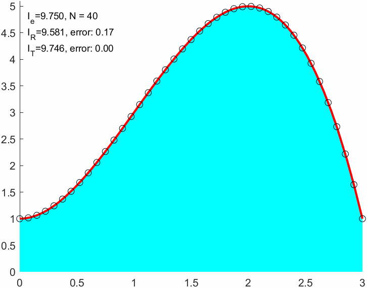

Exact numerical integration

The trapezoidal rule integrates linear polynomials exactly:

\int_a^b f\left(x\right)d\;x\approx \dfrac{b-a}{2}\left(f\left(a\right)+f\left(b\right)\right)

f = @(x)1+3*x;
a = 0; b = 3;
I1 = (f(a)+f(b))*(b-a)/2

I1 = 16.5000

I_exact = vpa(int(sym(f),a,b),5)

16.5

But there is a cheaper way...

We can evaluate the midpoint $\frac{\left(a+b\right)}{2}$ instead:

xm = (a+b)/2;
I1 = (b-a)*f(xm)

I1 = 16.5000

One function evaluation instead of 2!

This is exact because the error above the graph cancels the error below the graph!

Gauss quadrature rule

One rule to rule them all.

⚠ Note

This error cancelling property can be generalized so that

n

integration points integrate polynomials of degree

2n-1

exactly!

Gauss quadrature states for $x\in \left\lbrack 0,1\right\rbrack$

\boxed{ \int_0^1 p\left(x\right)\;d\;x\approx \sum_i^{\;} p\left(x_i \right)w_i }

\def\arraystretch{2.5} \begin{array}{cccc} \textrm{Gauss}\;\textrm{order} & \textrm{Polynomial}\;\textrm{order} & \textrm{Weights} & \textrm{Points}\\ 1 & 1 & 1 & \dfrac{1}{2}\\ 2 & 3 & \dfrac{1}{2} & \dfrac{1}{2}-\dfrac{\sqrt{3} }{6}\\ \; & \; & \dfrac{1}{2} & \dfrac{1}{2}+\dfrac{\sqrt{3} }{6}\\ 3 & 5 & \dfrac{5}{18} & \dfrac{1}{2}-\dfrac{\sqrt{3}\sqrt{5} }{10}\\ \; & \; & \dfrac{4}{9} & \dfrac{1}{2}\\ \; & \; & \dfrac{5}{18} & \dfrac{1}{2}+\dfrac{\sqrt{3}\sqrt{5} }{10} \end{array}

Example:

syms x
p = @(x) x;
I_e  = int(sym(p),x,0,1)

\frac{1}{2}

gp = 1/2; gw = 1;
I_G = p(gp)*gw

I_G = 0.5000

Ok, not a big deal, after all, even the Riemann sum is exact for linear polynomials.

How about a third order polynomial using only two function evaluations?

\int_0^1 1+3x-{3x}^3 \;d\;x=\sum_i^2 f\left(x_i \right)w_i

where $x_1 =\frac{1}{2}-\frac{\sqrt{3} }{6}$ and $x_2 =\frac{1}{2}+\frac{\sqrt{3} }{6}$ and $w_{1,2} =\frac{1}{2}$

p = @(x)1+3*x.^2-3*x.^3;

gp = [1/2-sym(sqrt(3))/6, 1/2+sym(sqrt(3))/6]

\left(\begin{array}{cc} \frac{1}{2}-\frac{\sqrt{3} }{6} & \frac{\sqrt{3} }{6}+\frac{1}{2} \end{array}\right)

gw = sym([1/2, 1/2])

\left(\begin{array}{cc} \frac{1}{2} & \frac{1}{2} \end{array}\right)

I_Gauss = p(gp(1))*gw(1) + p(gp(2))*gw(2)

\frac{3\,{ {\left(\frac{\sqrt{3} }{6}-\frac{1}{2}\right)} }^2 }{2}+\frac{3\,{ {\left(\frac{\sqrt{3} }{6}+\frac{1}{2}\right)} }^2 }{2}+\frac{3\,{ {\left(\frac{\sqrt{3} }{6}-\frac{1}{2}\right)} }^3 }{2}-\frac{3\,{ {\left(\frac{\sqrt{3} }{6}+\frac{1}{2}\right)} }^3 }{2}+1

vpa(I_Gauss)

1.25

simplify(I_Gauss)

\frac{5}{4}

xnod = linspace(0,1,50);
I_trapz = vpa(trapz(xnod,p(xnod)))

1.2498958767180341524364847980008

I_exact = int(sym(p),x,0,1)

\frac{5}{4}

figure; hold on
area([0,1/2],[1,1]*p(gp(1)),'FaceColor','c');
area([1/2,1],[1,1]*p(gp(2)),'FaceColor','c');
fplot(p,[0,1], 'r', 'LineWidth',2)
plot(gp,p(gp),'k*')
plot([0.5, 0.5], [0, p(gp(2))], '-k')

The figure visualizes the Gauss integration rule in action. The cyan and white areas between the curves are cancelling out!

Higher order Gauss integration will not make the integral any more accurate, the computed value will be the same. We will just be wasting computational power.

Non trivial integrals

Note that Gauss is not going to exactly integrade other functions in general.

Example - A tricky integral

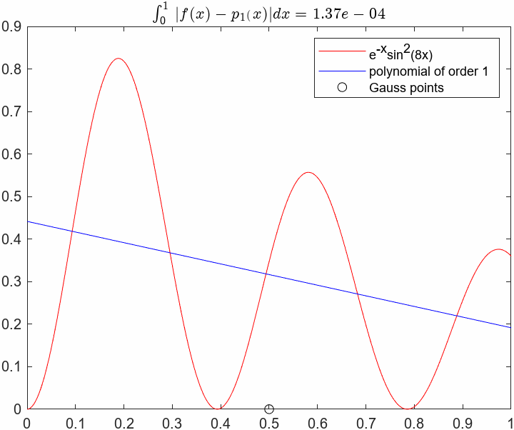
Let's say we need to integrate the function

f\left(x\right)=\dfrac{1}{\sqrt{\sin \left(x\right)} }\;\;\textrm{for}\;x\in \left\lbrack 0,1\right\rbrack

The resulting integral

\int_0^1 \dfrac{1}{\sqrt{\sin \left(x\right)} }\;\;d\;x

is non-elementary.

clear
syms x
f(x) = 1/sqrt(sin(x))

figure
fplot(f,[0,1],'k','LineWidth',2)
axis([0,1,0,10])
xnod = linspace(0.01,1,1000);
ynod = double(f(xnod));
hold on
area(xnod,ynod,'FaceColor','c','EdgeColor','none')

int(f)

-2\,{\textrm{F} }\left.\left(\frac{\pi }{4}-\frac{x}{2}\right|2\right)

int(f,x,0,1)

2\,{\textrm{F} }\left.\left(\frac{\pi }{4}\right|2\right)-2\,{\textrm{F} }\left.\left(\frac{\pi }{4}-\frac{1}{2}\right|2\right)

We can of course use the built-in numerical integration to solve this

I_e = vpaintegral(f,x,0,1)

2.03481

We can apply Gauss integration using the tabulated values from above:

f = matlabFunction(f);

[gp, gw] = GaussTable(3);
I_G = f(gp)*gw

I_G = 1.7857

error_Gauss = I_e-I_G

0.24915270426505561895957896467735

We can see that 3 Gauss points is not enough to sufficiently integrate this function. We need more points!

Let's go down the rabit hole, there exists quadrature tables containing Gauss points for the typical range $\left\lbrack -1,1\right\rbrack$ but there are also several algorithms for computing Gauss points for any Gauss order. Well use the well known Golub-Welsh algorithm taken from L. N. Trefethen, Spectral Methods in Matlab, SIAM, 2000 p.129

f = @(x)1./sqrt(sin(x))

a = 0; b = 1;
N = 17;
[gp, gw] = gauss(N, a, b);
I_G = vpa((b-a)*f(gp)*gw)

1.98504875258198065779424723587

error_Gauss = abs(I_e-I_G)

0.049756527078594875446171386101923

xnod = linspace(a+0.01,b,N)';
I_T = trapz(xnod,f(xnod))

I_T = 1.9312

error_Trapz = abs(I_e-I_T)

0.10356888582765996775769679061341

We can plot the error versus the number of evaluations

a = 0; b = 1;
err_G = []; err_Trapz = [];
NP = [2,4,8,16,32,64,128,256];
for N = NP
    [gp, gw] = gauss(N, a, b);
    I_G = vpa((b-a)*f(gp)*gw);
    xnod = linspace(a+0.003,b,N)';
    I_T = trapz(xnod,f(xnod));

    error_Gauss = abs(I_e-I_G);
    error_Trapz = abs(I_e-I_T);

    err_G(end+1) = error_Gauss;
    err_Trapz(end+1) = error_Trapz;
end

figure;
plot(NP,err_G,'-o','DisplayName','Gauss error'); hold on
plot(NP,err_Trapz,'-x','DisplayName','Trapz error')
gca().set(XScale='log',YScale='log')
legend show
xlabel('N evaluation points')
ylabel('Absolute error')
grid on
xticks(NP)
xticklabels({'2','4','8','16','32','64','128','256'})

We can see that both methods converge to the numerical integral computed by vpaintegral. The trapezoidal integral here is volotile, its lower bound needs to be adjusted to avoid the obious error division by zero. The computation thus depends on the choice of the new lower bound, and for a careful choice of lower bound we can get the trapezoidal method to outperform Gauss for some intermediate number of evaluations. The problem is that we cannot know this value ahead of time and thus the method is not very suitable for this situation.

Example - A sinusoidal

u\left(x\right)=2\;x\;\sin \left(2\;\pi \;x\right)+3\;\;\textrm{for}\;x\in \left\lbrack -0\ldotp 3,0\ldotp 9\right\rbrack

If we want to apply Gaussian quadrature here, we need to make a variable change to integrate over ranges other that $\left\lbrack 0,1\right\rbrack$ .

We can take any range $x\in \left\lbrack a,\;b\right\rbrack$ and map it to the range $\xi \in \left\lbrack 0,1\right\rbrack$ using iso-parametric mapping:

$x\left(\xi \right):=\left(1-\xi \right)a+\xi b$ and its derivative (or map) $\frac{d\;x}{d\;\xi }=b-a$ then we have

\int_a^b f\left(x\right)\;d\;x\;=\int_0^1 f\left(x\left(\xi \right)\right)\;\dfrac{d\;x}{d\;\xi }\;d\xi =\left(b-a\right)\int_0^1 f\left(x\left(\xi \right)\right)\;d\;\xi

and using Gauss quadrature approximation we have

\left(b-a\right)\int_0^1 f\left(x\left(\xi \right)\right)\;d\;\xi \approx \left(b-a\right)\sum_i^N f\left(x_i \right)w_i

clear
syms x
u(x) = 2*x*sin(2*pi*x)+3

a = -0.3; b = 0.9;
figure
fplot(u,[a,b],'k','LineWidth',2)
% axis([a,b,0,10])
xnod = linspace(a,b,1000);
ynod = double(u(xnod));
hold on
area(xnod,ynod,'FaceColor','c','EdgeColor','none')

I_e = int(u,x,a,b);
I_e = vpa(I_e)

3.4161461898582861156669109907739

And now let's approximate it using Gauss quadrature

f = matlabFunction(u);
N = 8;
[gp, gw] = gauss(N, a, b);
I_G = vpa((b-a)*f(gp)*gw)

3.4161461860196071782524995796848

error_Gauss = I_e-I_G

0.0000000038386789374144114110890740595862

xnod = linspace(a,b,N)';
I_T = vpa(trapz(xnod,f(xnod)))

3.437977129365528128346340963617

error_Trapz = I_e-I_T

-0.021830939507242012679429972843084

Error analysis

error.N = [2,4,8,16,32,64,128,256].';
error.Gauss = zeros(length(error.N),1);
error.Trapz = zeros(length(error.N),1);

for i = 1:length(error.N)
    N = error.N(i);
    xnod = linspace(a,b,N)';
    I_Trapz = trapz(xnod,f(xnod)); % Matlab built in trapezoidal integral
    
    [gp, gw] = gauss(N, a, b);
    I_Gauss = (b-a)*f(gp)*gw;
    
    error_Gauss = abs(I_e-I_Gauss);
    error_Trapz = abs(I_e-I_Trapz);
    
    error.Gauss(i) = error_Gauss;
    error.Trapz(i) = error_Trapz;
    
end
figure; hold on
plot(error.N, error.Gauss,'-o')
plot(error.N, error.Trapz,'-o')
grid on
set(gca,'xscale','log','yscale','log')
legend('Gauss','Trapz')
xlabel('N evaluation points')
ylabel('Absolute error')
xticks(error.N)
xticklabels({'2','4','8','16','32','64','128','256'})

Here we see that Gauss reaches the same precision as vpaintegral after 16 function evaluations.

Gauss visualized

Here is a visualization of the Gauss integration method for the function

f(x) = 2x \sin(12x)+3

for $x \in [-0.3, 0.9]$

Deriving the Gaussian quadrature rule

We can integrate the definite integral with limits by the approximation

\int_0^1 f\left(x\right)\;\textrm{dx}\approx \sum_i^n f\left(x_i \right)w_i

Now the Gaussian quadrature rule works by evaluating the function $f$ at some special points $x_i$ and multiplying by some special weights $w_i$ , the linear combination will result in an approximate integral that for a certain polynomial is exact as $n$ integration points integrate polynomials of degree $2n-1$ exactly!

When $f\left(x\right)$ is not a polynomial function, we still can approximate the integral by in a sense choosing the closest matching polynomial of the type $p\left(x\right)=a_0 +a_1 x+a_2 x^2 +\ldotp \ldotp \ldotp +a_n x^n$ and the corresponding Gauss quadrature rule to integrate this polynomial exactly.

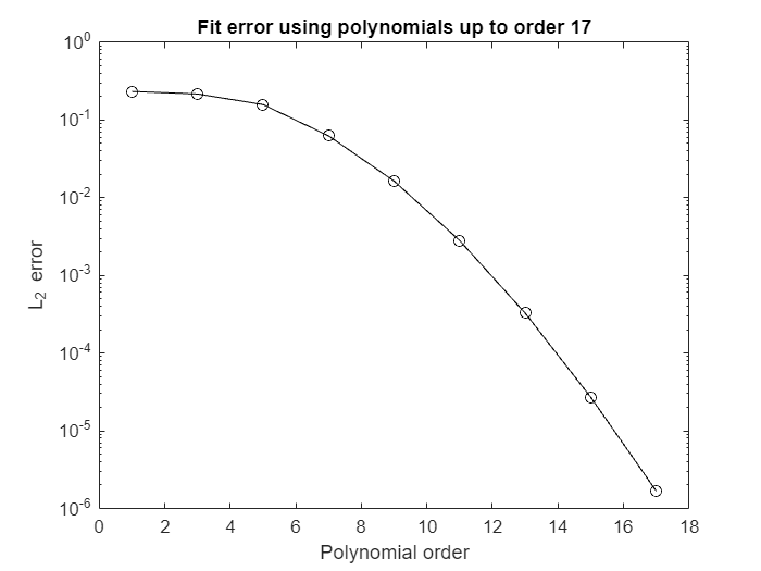
These special points and weights can be found by many ways where the Golub-Welsch algorithm is implemented in the gauss.m function, but we shall here take a look at another which is arguably simpler to explain.

⚠ Note

Most common integration limits are

-1

1

since they are symmetric around 0 and since the Gauss points are roots to the Legendre polynomials in this range. The reason we use 0 to 1 throughout this material is because of some unexplainable preference by the author.

For a certain approximation, e.g., the linear

\hat{f} \left(x\right)=a_0 +a_1 x

we have

w_1 \hat{f_i } \left(x_i \right)=\int_0^1 \hat{f_i } \left(x_i \right)\textrm{dx}

with $\hat{f_1 } =1,\hat{f_2 } =x$

This yields a system of equations

\def\arraystretch{2.0} \left\lbrace \begin{array}{ll} w_1 \cdot 1=\int_0^1 1\textrm{dx} & \Rightarrow w_1 =1\\ w_1 \cdot x_1 =\int_0^1 \textrm{xdx} & \Rightarrow x_1 = 1/2 \end{array}\right.

This also works for higher order approximations, e.g., cubic. Note we need polynomial functions which contain even terms since the points and weights are associated with the unknown coefficients $a_i$

\hat{f} \left(x\right)=a_0 +a_1 x+a_2 x^2 +a_3 x^3

with $\hat{f_1 } =1,\;\hat{f_2 } =x,\;\hat{f_3 } =x^2 ,\;\hat{f_4 } =x^3$

from which we form

w_1 \hat{f_i } \left(x_1 \right)+w_2 \hat{f_i } \left(x_2 \right)=\int_0^1 \hat{f_i } \left(x\right)\textrm{dx}

\def\arraystretch{2.0} \left\lbrace \begin{array}{c} i=1:\;\;\;\;\;\;\;\;\;\;\;\;\;\;\;\;\;\;\;w_1 +w_2 =\int_0^1 1\textrm{dx}=1\\ i=2:\;\;\;\;\;\;\;w_1 x_1 +w_2 x_2 =\int_0^1 \textrm{xdx}=1/2\\ i=3:\;\;\;\;\;w_1 x_1^2 +w_2 x_2^2 =\int_0^1 x^2 \textrm{dx}=1/3\\ i=4:\;\;\;\;\;w_1 x_1^3 +w_2 x_2^3 =\int_0^1 x^3 \textrm{dx}=1/4 \end{array}\right.

Now we could solve this symbolically, below, but we shall also see how to solve this system of non-linear equations using numerically using Newton's method.

syms w1 w2 x1 x2 x

ekv = [w1    + w2        == int(1,x,0,1)
       w1*x1 + w2*x2     == int(x,x,0,1)
       w1*x1^2 + w2*x2^2 == int(x^2,x,0,1)
       w1*x1^3 + w2*x2^3 == int(x^3,x,0,1)]

[w1 w2 x1 x2] = solve(ekv, [w1 w2 x1 x2])

We get two solutions:

\bm w_1= \left(\begin{array}{c} 1/2\\ 1/2 \end{array}\right)

\bm w_2= \left(\begin{array}{c} 1/2\\ 1/2 \end{array}\right)

\bm x_1= \left(\begin{array}{c} \frac{\sqrt{3}}{6}+\frac{1}{2}\\ \frac{1}{2}-\frac{\sqrt{3}}{6} \end{array}\right)

\bm x_2= \left(\begin{array}{c} \frac{1}{2}-\frac{\sqrt{3}}{6}\\ \frac{\sqrt{3}}{6}+\frac{1}{2} \end{array}\right)

Solving non-linear system of equations

The Newton method states

{\mathit{\mathbf{x} } }^{k+1} ={\mathit{\mathbf{x} } }^k -{\mathit{\mathbf{J} }\left({\mathit{\mathbf{x} } }^k \right)}^{-1} \mathit{\mathbf{f} }\left({\mathit{\mathbf{x} } }^k \right)

where

\mathit{\mathbf{J} }=\left\lbrack \begin{array}{cccc} \dfrac{\partial f_1 }{\partial x_1 } & \dfrac{\partial f_1 }{\partial x_2 } & \cdots & \dfrac{\partial f_1 }{\partial x_n }\\ \dfrac{\partial f_2 }{\partial x_1 } & \dfrac{\partial f_2 }{\partial x_2 } & \cdots & \dfrac{\partial f_2 }{\partial x_n }\\ \vdots & \vdots & \ddots & \vdots \\ \dfrac{\partial f_n }{\partial x_1 } & \dfrac{\partial f_n }{\partial x_2 } & \cdots & \dfrac{\partial f_n }{\partial x_n } \end{array}\right\rbrack

Now we rewrite this such that we can turn it into a linear system

\mathit{\mathbf{J} }\left({\mathit{\mathbf{x} } }^k \right)\left({\mathit{\mathbf{x} } }^{k+1} -{\mathit{\mathbf{x} } }^k \right)=-\mathit{\mathbf{f} }\left({\mathit{\mathbf{x} } }^k \right)

\mathbf{Ax}=\mathbf{b}

with $\mathbf{A}=\mathit{\mathbf{J} }\left({\mathit{\mathbf{x} } }^k \right)$ , $\mathbf{x}=\Delta \mathit{\mathbf{x} }=\left({\mathit{\mathbf{x} } }^{k+1} -{\mathit{\mathbf{x} } }^k \right)$ and $\mathbf{b}=-\mathit{\mathbf{f} }\left({\mathit{\mathbf{x} } }^k \right)$

We will also need initial values for $w_1 ,w_2 ,x_1 ,x_2$ , we will choose randomly such that they all are in the interval $\left\lbrack 0,1\right\rbrack$ .

syms w1 w2 x1 x2 x
f1 = w1 + w2 - int(1,x,0,1);
f2 = w1*x1 + w2*x2 - int(x,x,0,1);
f3 = w1*x1^2 + w2*x2^2 - int(x^2,x,0,1);
f3 = w1*x1^2 + w2*x2^2 - int(x^2,x,0,1);

J = [diff(f1,w1), diff(f1, w2), diff(f1, x1), diff(f1, x2)
     diff(f2,w1), diff(f2, w2), diff(f2, x1), diff(f2, x2)
     diff(f3,w1), diff(f3, w2), diff(f3, x1), diff(f3, x2)
     diff(f4,w1), diff(f4, w2), diff(f4, x1), diff(f4, x2)];

f = [f1
     f2
     f3
     f4];


% Going numeric here
J = matlabFunction(J);
f = matlabFunction(f);

w1 = rand; w2 = rand; x1 = rand; x2 = rand;

xold = [w1
        w2
        x1
        x2];

for i = 1:1000
    xold = [w1
            w2
            x1
            x2];
    Jnew = J(w1,w2,x1,x2);
    fnew = f(w1,w2,x1,x2);
    xd = Jnew\-fnew;
    xnew = xold + xd;
    
    w1 = xnew(1); w2 = xnew(2); x1 = xnew(3); x2 = xnew(4);
    
    eps = norm(xold - xnew)
    if eps < 1e-12 %stop at an arbitrary precision
        break; 
    end
end

Depending on the initial values, the algorithm will take a different amount of iterations to converge below the set tolerance.

eps = 0.5225
eps = 0.0709
eps = 0.0195
eps = 6.9134e-04
eps = 2.6636e-07
eps = 1.1066e-13

The converged numerical values:

w1 = 0.5000
w2 = 0.5000
x1 = 0.2113
x2 = 0.7887

Code snippets

function [gp, gw] = GaussTable(n)

    switch n
        case 1
            gp = 0.5;
            gw = 1;
        case 2
            gp = [0.5-sqrt(3)/6
                  0.5+sqrt(3)/6]';
            gw = [0.5
                  0.5];
        case 3
            gp = [0.5-sqrt(3)*sqrt(5)/10
                  0.5
                  0.5+sqrt(3)*sqrt(5)/10]';
            gw = [5/18
                  4/9
                  5/18];
    end

end

function [x, w, A] = gauss(n, a, b)
    
    %------------------------------------------------------------------------------
    % gauss.m
    %------------------------------------------------------------------------------
    %
    % Purpose:
    %
    % Generates abscissas and weights on I = [ a, b ] (for Gaussian quadrature).
    %
    % Implementation of the Golub-Welsch algorithm
    % https://en.wikipedia.org/wiki/Gaussian_quadrature#The_Golub-Welsch_algorithm
    %
    % Syntax:
    %
    % [x, w, A] = gauss(n, a, b);
    %
    %
    % Input:
    %
    % n    integer    Number of quadrature points.
    % a    real       Left endpoint of interval.
    % b    real       Right endpoint of interval.
    %
    %
    % Output:
    %
    % x    real       Quadrature points.
    % w    real       Weigths.
    % A    real       Area of domain.
    %------------------------------------------------------------------------------
    
    
    % 3-term recurrence coefficients:
    n = 1:(n - 1);
    beta = 1 ./ sqrt(4 - 1 ./ (n .* n));
    
    % Jacobi matrix:
    J = diag(beta, 1) + diag(beta, -1); 
    
    
    % Eigenvalue decomposition:
    
    %
    % e-values are used for abscissas, whereas e-vectors determine weights.
    %
    
    [V, D] = eig(J);
    x = diag(D);
    
    
    % Size of domain:
    A = b - a;
    
    
    % Change of interval:
    
    %
    % Initally we have I0 = [ -1, 1 ]; now one gets I = [ a, b ] instead.
    %
    % The abscissas are Legendre points.
    %
    
    if ~(a == -1 && b == 1)
      x = 0.5 * A * x + 0.5 * (b + a);
    end
    
    
    % Weigths:
    w = V(1, :) .* V(1, :);
    w = w';
    x=x';
end