Download this page as a Matlab LiveScript
Table of contents
Solving differential equations using Galerkin
VIDEO
Piecewise approximation
VIDEO
Example
{ − d 2 u d x = x 2 for x ∈ [ 0 , 1 ] u ( 0 ) = − 1 d u d x ( 1 ) = − 2
\def\arraystretch{2.0}
\left\lbrace \begin{array}{ll}
-\dfrac{d^2 u}{d\;x}=x^2 & \textrm{for}\;x\in \left\lbrack 0,1\right\rbrack \\
u\left(0\right)=-1 & \;\\
\dfrac{d\;u}{d\;x}\left(1\right)=-2 & \;
\end{array}\right.
⎩ ⎨ ⎧ − d x d 2 u = x 2 u ( 0 ) = − 1 d x d u ( 1 ) = − 2 for x ∈ [ 0 , 1 ] Weak form:
∫ 0 1 − d 2 u d x v d x = ∫ 0 1 x 2 v d x \int_0^1 -\dfrac{d^2 u}{d\;x}\;v\;dx=\int_0^1 x^2 v \;dx ∫ 0 1 − d x d 2 u v d x = ∫ 0 1 x 2 v d x ⇒ ∫ 0 1 d u d x d v d x d x = ∫ 0 1 x 2 v d x + [ d u d x ( x ) v ( x ) ] 0 1 \Rightarrow \int_0^1 \dfrac{d\;u}{dx}\;\dfrac{d\;v}{d\;x}\;d\;x=\int_0^1 x^2 v \; dx + {\left\lbrack \dfrac{d\;u}{d\;x}\left(x\right)\;v\left(x\right)\right\rbrack }_0^1 ⇒ ∫ 0 1 d x d u d x d v d x = ∫ 0 1 x 2 v d x + [ d x d u ( x ) v ( x ) ] 0 1 Approximation using Galerkin
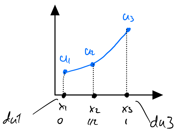
du1 = d u d x ( 0 ) , du2 = d u d x ( 1 ) = − 2 , u 1 = − 1 \textrm{du1}=\dfrac{d\;u}{d\;x}\left(0\right),\;\;\textrm{du2}=\dfrac{d\;u}{d\;x}\left(1\right)=-2,\;u_1 =-1 du1 = d x d u ( 0 ) , du2 = d x d u ( 1 ) = − 2 , u 1 = − 1 Approximate using one quadratic element on the whole domain
Quadratic basis functions: For x ∈ [ 0 , 1 ] x\in \left\lbrack 0,1\right\rbrack \; x ∈ [ 0 , 1 ]
φ 1 = 2 ( x − 1 ) ( x − 1 / 2 ) φ 2 = − 4 x ( x − 1 ) φ 3 = 2 x ( x − 1 / 2 )
\def\arraystretch{1.5}
\begin{array}{l}
\varphi_1 =2\left(x-1\right)\left(x-1/2\right)\\
\varphi_2 =-4x\left(x-1\right)\\
\varphi_3 =2x\left(x-1/2\right)
\end{array}
φ 1 = 2 ( x − 1 ) ( x − 1/2 ) φ 2 = − 4 x ( x − 1 ) φ 3 = 2 x ( x − 1/2 ) The solution is then approximated by
U ( x ) = ∑ i = 1 3 u i φ i U\left(x\right)=\sum_{i=1}^3 u_i {\;\varphi }_i U ( x ) = i = 1 ∑ 3 u i φ i and the derivate is given by
d U d x = d d x ( ∑ u i φ i ( x ) ) = ∑ u i d φ i d x \dfrac{d\;U}{d\;x}=\dfrac{d}{d\;x}\left(\sum_{\;} u_{i\;} \varphi_i \left(x\right)\right)=\sum_{\;} u_i \;\dfrac{d{\;\varphi }_i }{d\;x} d x d U = d x d ( ∑ u i φ i ( x ) ) = ∑ u i d x d φ i Insert the approximation into the weak form, replacing v v\; v φ \varphi φ d v d x \frac{d\;v}{d\;x} d x d v d φ d x \frac{d\;\varphi }{d\;x} d x d φ
∫ 0 1 ∑ d φ i d x u i d φ j d x d x = ∫ 0 1 x 2 φ j d x + d u d x ( 1 ) φ ( 1 ) ⏟ − 2 \int_0^1 \sum_{\;} \dfrac{d\;\varphi_i }{d\;x}\;u_i \;\dfrac{d\;\varphi_j }{d\;x}\;d\;x=\int_0^1 x^2 \;\varphi_j \;d\;x+\underset{-2}{\underbrace{\dfrac{d\;u}{d\;x}\left(1\right)\varphi \left(1\right)} } ∫ 0 1 ∑ d x d φ i u i d x d φ j d x = ∫ 0 1 x 2 φ j d x + − 2 d x d u ( 1 ) φ ( 1 ) Switch to Matlab to solve the equations.
clear
syms u1 u2 u3 x
phi(x) = [2 *(x-1 )*(x-1 /2 ) -4 *x*(x-1 ) 2 *x*(x-1 /2 )];
u = [u1; u2; u3];
dphi = diff(phi,x)( 4 x − 3 4 − 8 x 4 x − 1 ) \left(\begin{array}{ccc}
4\,x-3 & 4-8\,x & 4\,x-1
\end{array}\right) ( 4 x − 3 4 − 8 x 4 x − 1 ) syms du0
eqs = int(dphi*u*dphi,x,0 ,1 ) == int(x^2 *phi, x, 0 , 1 ) + phi(1 )*-2 - phi(0 )*du0;
eqs.'( 7 u 1 3 − 8 u 2 3 + u 3 3 = − du 0 − 1 60 16 u 2 3 − 8 u 1 3 − 8 u 3 3 = 1 5 u 1 3 − 8 u 2 3 + 7 u 3 3 = − 37 20 )
\def\arraystretch{2.5}
\left(\begin{array}{c}
\dfrac{7\,u_1 }{3}-\dfrac{8\,u_2 }{3}+\dfrac{u_3 }{3}=-{\textrm{du} }_0 -\dfrac{1}{60}\\
\dfrac{16\,u_2 }{3}-\dfrac{8\,u_1 }{3}-\dfrac{8\,u_3 }{3}=\dfrac{1}{5}\\
\dfrac{u_1 }{3}-\dfrac{8\,u_2 }{3}+\dfrac{7\,u_3 }{3}=-\dfrac{37}{20}
\end{array}\right)
⎝ ⎛ 3 7 u 1 − 3 8 u 2 + 3 u 3 = − du 0 − 60 1 3 16 u 2 − 3 8 u 1 − 3 8 u 3 = 5 1 3 u 1 − 3 8 u 2 + 3 7 u 3 = − 20 37 ⎠ ⎞ Set the boundary condition, the known nodal value:
u1 = -1 Here we have two alternatives, either reduce the equations to two, by eliminating the equation where u 1 u_1 u 1 d u d x ( 0 ) \frac{d\;u}{d\;x}\left(0\right) d x d u ( 0 )
[u2, u3] = solve(subs(eqs(2 :3 )),[u2, u3] )U = simplify(subs(phi*u))− 3 x 2 20 − 8 x 5 − 1 -\dfrac{3\,x^2 }{20}-\dfrac{8\,x}{5}-1 − 20 3 x 2 − 5 8 x − 1 syms ue(x)
DE = -diff(ue,x,2 ) == x^2 ;
du = diff(ue,x,1 );
BC = [ue(0 )==-1 , du(1 )==-2 ];
ue = dsolve(DE,BC)− x 4 12 − 5 x 3 − 1 -\dfrac{x^4 }{12}-\dfrac{5\,x}{3}-1 − 12 x 4 − 3 5 x − 1 figure
fplot(ue, [0 ,1 ],'r' ,'DisplayName' ,'Exact solution' ); hold on
fplot(U,[0 ,1 ],'b' ,'DisplayName' ,'Approximation' )
plot ([0 ,0.5 ,1 ],[u1,u2,u3],'ob' ,'DisplayName' ,'u_i' )
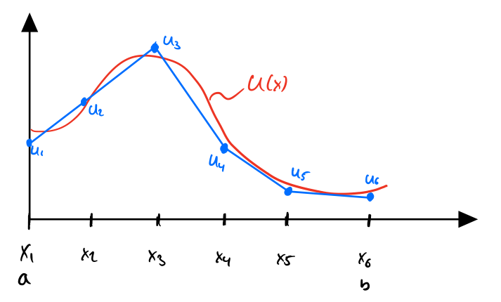
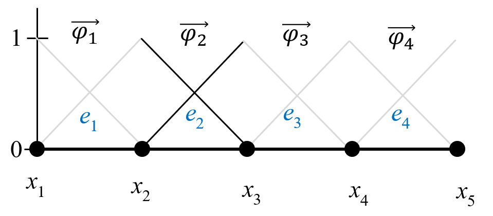
legend showInstead of approximating the solution using one trial function, we can split the domain into N N N
In this example we want to find all 6 nodal values u i u_i u i
∫ a b ( U − u ) φ i d x = 0 \int_a^b \left(U-u\right)\varphi_i dx=0 ∫ a b ( U − u ) φ i d x = 0 In order to solve this we need to define φ i ( x ) \varphi_i \left(x\right) φ i ( x )
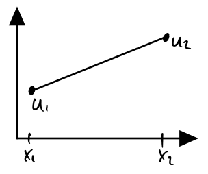
We can define a polynomial function using its nodal values:
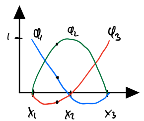
U ( x ) = x 2 − x x 2 − x 1 u 1 + x − x 1 x 2 − x 1 = φ 1 u 1 + φ 1 u 1 U\left(x\right)=\dfrac{x_2 -x}{x_2 -x_1 }u_1 +\dfrac{x-x_1 }{x_2 -x_1 }=\varphi_1 u_1 +\varphi_1 u_1 U ( x ) = x 2 − x 1 x 2 − x u 1 + x 2 − x 1 x − x 1 = φ 1 u 1 + φ 1 u 1 The definition of a nodal basis function: Let the i'th basis function be equal to 1 in the i'th node and 0 in all other nodes.
φ j ( x i ) = { 1 if i = j 0 if i ≠ j \varphi_j \left(x_i \right)=\left\lbrace \begin{array}{ll}
1 & \textrm{if}\;i=j\\
0 & \textrm{if}\;i\not= j
\end{array}\right. φ j ( x i ) = { 1 0 if i = j if i = j To derive the basis functions use the definition and make the ansatz:
φ ( x ) = c 1 + c 2 x \varphi \left(x\right)=c_1 +c_2 x φ ( x ) = c 1 + c 2 x φ 1 ( 0 ) = c 1 + c 2 ⋅ 0 = 1 φ 1 ( 1 ) = c 1 + c 2 ⋅ 1 = 0 φ 2 ( 0 ) = c 1 + c 2 ⋅ 0 = 0 φ 2 ( 1 ) = c 1 + c 2 ⋅ 1 = 1
\def\arraystretch{1.5}
\begin{array}{l}
\varphi_1 \left(0\right)=c_1 +c_2 \cdot 0=1\\
\varphi_1 \left(1\right)=c_1 +c_2 \cdot 1=0\\
\varphi_2 \left(0\right)=c_1 +c_2 \cdot 0=0\\
\varphi_2 \left(1\right)=c_1 +c_2 \cdot 1=1
\end{array}
φ 1 ( 0 ) = c 1 + c 2 ⋅ 0 = 1 φ 1 ( 1 ) = c 1 + c 2 ⋅ 1 = 0 φ 2 ( 0 ) = c 1 + c 2 ⋅ 0 = 0 φ 2 ( 1 ) = c 1 + c 2 ⋅ 1 = 1 or on matrix form
[ 1 x 1 1 x 2 ] [ c 11 c 21 ] = [ 1 0 ] \left\lbrack \begin{array}{cc}
1 & x_1 \\
1 & x_2
\end{array}\right\rbrack \left\lbrack \begin{array}{c}
c_{11} \\
c_{21}
\end{array}\right\rbrack =\left\lbrack \begin{array}{c}
1\\
0
\end{array}\right\rbrack [ 1 1 x 1 x 2 ] [ c 11 c 21 ] = [ 1 0 ] [ 1 x 1 1 x 2 ] [ c 12 c 22 ] = [ 0 1 ] \left\lbrack \begin{array}{cc}
1 & x_1 \\
1 & x_2
\end{array}\right\rbrack \left\lbrack \begin{array}{c}
c_{12} \\
c_{22}
\end{array}\right\rbrack =\left\lbrack \begin{array}{c}
0\\
1
\end{array}\right\rbrack [ 1 1 x 1 x 2 ] [ c 12 c 22 ] = [ 0 1 ]
or
[ 1 x 1 1 x 2 ] ⏟ A [ c 11 c 12 c 21 c 22 ] ⏟ C = [ 1 0 0 1 ] ⏟ I ⇒ C = A − 1 I \underset{\mathit{\mathbf{A}}}{\underbrace{\left\lbrack \begin{array}{cc}
1 & x_1 \\
1 & x_2
\end{array}\right\rbrack } } \underset{\mathit{\mathbf{C}}}{\underbrace{\left\lbrack \begin{array}{cc}
c_{11} & c_{12} \\
c_{21} & c_{22}
\end{array}\right\rbrack } } =\underset{\mathit{\mathbf{I}}}{\underbrace{\left\lbrack \begin{array}{cc}
1 & 0\\
0 & 1
\end{array}\right\rbrack } } \Rightarrow \mathit{\mathbf{C}}={\mathit{\mathbf{A}}}^{-1} \mathit{\mathbf{I}} A [ 1 1 x 1 x 2 ] C [ c 11 c 21 c 12 c 22 ] = I [ 1 0 0 1 ] ⇒ C = A − 1 I φ ( x ) = [ 1 x ] C \varphi \left(x\right)=\left\lbrack 1\;x\right\rbrack \mathit{\mathbf{C}} φ ( x ) = [ 1 x ] C syms x1 x2 x
A = [1 x1
1 x2]( 1 x 1 1 x 2 )
\left(\begin{array}{cc}
1 & x_1 \\
1 & x_2
\end{array}\right)
( 1 1 x 1 x 2 ) C = A\eye (2 )( − x 2 x 1 − x 2 x 1 x 1 − x 2 1 x 1 − x 2 − 1 x 1 − x 2 )
\def\arraystretch{2.5}
\left(\begin{array}{cc}
-\dfrac{x_2 }{x_1 -x_2 } & \dfrac{x_1 }{x_1 -x_2 }\\
\dfrac{1}{x_1 -x_2 } & -\dfrac{1}{x_1 -x_2 }
\end{array}\right)
⎝ ⎛ − x 1 − x 2 x 2 x 1 − x 2 1 x 1 − x 2 x 1 − x 1 − x 2 1 ⎠ ⎞ phi = simplify([1 x]*C)( x − x 2 x 1 − x 2 − x − x 1 x 1 − x 2 ) \left(\begin{array}{cc}
\dfrac{x-x_2 }{x_1 -x_2 } & -\dfrac{x-x_1 }{x_1 -x_2 }
\end{array}\right) ( x 1 − x 2 x − x 2 − x 1 − x 2 x − x 1 ) For quadratic make the ansatz: φ ( x ) = c 1 + c 2 x + c 3 x 2 \varphi \left(x\right)=c_1 +c_2 x+c_3 x^2 φ ( x ) = c 1 + c 2 x + c 3 x 2
φ 1 ( 0 ) = c 1 + c 2 ⋅ 0 + c 3 ⋅ 0 2 = 1 φ 1 ( 1 / 2 ) = c 1 + c 2 ⋅ 1 / 2 + c 3 ⋅ ( 1 / 2 ) 2 = 0 φ 1 ( 1 ) = c 1 + c 2 ⋅ 1 + c 3 ⋅ 1 2 = 0 φ 2 ( 0 ) = c 1 + c 2 ⋅ 0 + c 3 ⋅ 0 2 = 0 φ 2 ( 1 / 2 ) = c 1 + c 2 ⋅ 1 / 2 + c 3 ⋅ ( 1 / 2 ) 2 = 1 φ 2 ( 1 ) = c 1 + c 2 ⋅ 1 + c 3 ⋅ 1 2 = 0 φ 3 ( 0 ) = c 1 + c 2 ⋅ 0 + c 3 ⋅ 0 2 = 0 φ 3 ( 1 / 2 ) = c 1 + c 2 ⋅ 1 / 2 + c 3 ⋅ ( 1 / 2 ) 2 = 0 φ 3 ( 1 ) = c 1 + c 2 ⋅ 1 + c 3 ⋅ 1 2 = 1
\def\arraystretch{1.5}
\begin{array}{l}
\varphi_1 \left(0\right)=c_1 +c_2 \cdot 0+c_3 \cdot 0^2 =1\\
\varphi_1 \left(1/2\right)=c_1 +c_2 \cdot 1/2+c_3 \cdot {\left(1/2\right)}^2 =0\\
\varphi_1 \left(1\right)=c_1 +c_2 \cdot 1+c_3 \cdot 1^2 =0\\
\\
\varphi_2 \left(0\right)=c_1 +c_2 \cdot 0+c_3 \cdot 0^2 = 0\\
\varphi_2 \left(1/2\right)=c_1 +c_2 \cdot 1/2+c_3 \cdot {\left(1/2\right)}^2 = 1\\
\varphi_2 \left(1\right)=c_1 +c_2 \cdot 1+c_3 \cdot 1^2 = 0\\
\\
\varphi_3 \left(0\right)=c_1 +c_2 \cdot 0+c_3 \cdot 0^2 = 0\\
\varphi_3 \left(1/2\right)=c_1 +c_2 \cdot 1/2+c_3 \cdot {\left(1/2\right)}^2 = 0\\
\varphi_3 \left(1\right)=c_1 +c_2 \cdot 1+c_3 \cdot 1^2 = 1\\
\end{array}
φ 1 ( 0 ) = c 1 + c 2 ⋅ 0 + c 3 ⋅ 0 2 = 1 φ 1 ( 1/2 ) = c 1 + c 2 ⋅ 1/2 + c 3 ⋅ ( 1/2 ) 2 = 0 φ 1 ( 1 ) = c 1 + c 2 ⋅ 1 + c 3 ⋅ 1 2 = 0 φ 2 ( 0 ) = c 1 + c 2 ⋅ 0 + c 3 ⋅ 0 2 = 0 φ 2 ( 1/2 ) = c 1 + c 2 ⋅ 1/2 + c 3 ⋅ ( 1/2 ) 2 = 1 φ 2 ( 1 ) = c 1 + c 2 ⋅ 1 + c 3 ⋅ 1 2 = 0 φ 3 ( 0 ) = c 1 + c 2 ⋅ 0 + c 3 ⋅ 0 2 = 0 φ 3 ( 1/2 ) = c 1 + c 2 ⋅ 1/2 + c 3 ⋅ ( 1/2 ) 2 = 0 φ 3 ( 1 ) = c 1 + c 2 ⋅ 1 + c 3 ⋅ 1 2 = 1
which leads to the matrix system
[ 1 x 1 x 1 2 1 x 2 x 2 2 1 x 3 x 3 3 ] [ c 11 c 12 c 13 c 21 c 22 c 23 c 31 c 32 c 33 ] = [ 1 0 0 0 1 0 0 0 1 ] \left\lbrack \begin{array}{ccc}
1 & x_1 & x_1^2 \\
1 & x_2 & x_2^2 \\
1 & x_3 & x_{\;3}^3
\end{array}\right\rbrack \left\lbrack \begin{array}{ccc}
c_{11} & c_{12} & c_{13} \\
c_{21} & c_{22} & c_{23} \\
c_{31} & c_{32} & c_{33}
\end{array}\right\rbrack =\left\lbrack \begin{array}{ccc}
1 & 0 & 0\\
0 & 1 & 0\\
0 & 0 & 1
\end{array}\right\rbrack ⎣ ⎡ 1 1 1 x 1 x 2 x 3 x 1 2 x 2 2 x 3 3 ⎦ ⎤ ⎣ ⎡ c 11 c 21 c 31 c 12 c 22 c 32 c 13 c 23 c 33 ⎦ ⎤ = ⎣ ⎡ 1 0 0 0 1 0 0 0 1 ⎦ ⎤ φ ( x ) = [ 1 x x 2 ] C \varphi \left(x\right)=\left\lbrack 1\;\;x\;\;x^2 \right\rbrack \mathit{\mathbf{C}} φ ( x ) = [ 1 x x 2 ] C syms x1 x2 x3 x
A = [1 x1 x1^2
1 x2 x2^2
1 x3 x3^2 ];
C = A\eye (3 );
phi = simplify([1 x x^2 ]*C).'φ ( x ) = ( ( x − x 2 ) ( x − x 3 ) ( x 1 − x 2 ) ( x 1 − x 3 ) − ( x − x 1 ) ( x − x 3 ) ( x 1 − x 2 ) ( x 2 − x 3 ) ( x − x 1 ) ( x − x 2 ) ( x 1 − x 3 ) ( x 2 − x 3 ) ) for x ∈ [ x 1 , x 2 ]
\def\arraystretch{2.5}
\boldsymbol \varphi(x) =
\left(\begin{array}{c}
\dfrac{ {\left(x-x_2 \right)}\,{\left(x-x_3 \right)} }{ {\left(x_1 -x_2 \right)}\,{\left(x_1 -x_3 \right)} }\\
-\dfrac{ {\left(x-x_1 \right)}\,{\left(x-x_3 \right)} }{ {\left(x_1 -x_2 \right)}\,{\left(x_2 -x_3 \right)} }\\
\dfrac{ {\left(x-x_1 \right)}\,{\left(x-x_2 \right)} }{ {\left(x_1 -x_3 \right)}\,{\left(x_2 -x_3 \right)} }
\end{array}\right)
\quad \text{for } x \in [x_1, x_2]
φ ( x ) = ⎝ ⎛ ( x 1 − x 2 ) ( x 1 − x 3 ) ( x − x 2 ) ( x − x 3 ) − ( x 1 − x 2 ) ( x 2 − x 3 ) ( x − x 1 ) ( x − x 3 ) ( x 1 − x 3 ) ( x 2 − x 3 ) ( x − x 1 ) ( x − x 2 ) ⎠ ⎞ for x ∈ [ x 1 , x 2 ] and for x 1 = 0 , x 2 = 1 / 2 , x 3 = 1 x_1 =0,x_2 =1/2,x_3 =1 x 1 = 0 , x 2 = 1/2 , x 3 = 1
subs(phi,[x1 x2 x3], [0 , 1 /2 , 1 ])φ ( x ) = ( 2 ( x − 1 ) ( x − 1 2 ) − 4 x ( x − 1 ) 2 x ( x − 1 2 ) ) for x ∈ [ 0 , 1 ]
\def\arraystretch{2.0}
\boldsymbol \varphi(x) =
\left(\begin{array}{c}
2\,{\left(x-1\right)}\,{\left(x-\dfrac{1}{2}\right)}\\
-4\,x\,{\left(x-1\right)}\\
2\,x\,{\left(x-\dfrac{1}{2}\right)}
\end{array}\right)
\quad \text{for } x \in [0, 1]
φ ( x ) = ⎝ ⎛ 2 ( x − 1 ) ( x − 2 1 ) − 4 x ( x − 1 ) 2 x ( x − 2 1 ) ⎠ ⎞ for x ∈ [ 0 , 1 ] Solve
{ − d 2 u d x 2 = 1 for x ∈ [ 1 , 3 ] u ( 1 ) = 2 d u d x ( 3 ) = − 1
\def\arraystretch{2.0}
\left\lbrace \begin{array}{ll}
-\dfrac{d^2u}{dx^2}=1 & \textrm{for}\;x\in \left\lbrack 1,3\right\rbrack \\
u\left(1\right)=2 & \\
\dfrac{d\;u}{d\;x}\left(3\right)=-1 &
\end{array}\right.
⎩ ⎨ ⎧ − d x 2 d 2 u = 1 u ( 1 ) = 2 d x d u ( 3 ) = − 1 for x ∈ [ 1 , 3 ] using 4 linear elements.
Solution : Weak form:
∫ 1 3 d u d x d v d x d x = ∫ 1 3 1 ⋅ v d x + [ d u d x v ] 1 3 \int_1^3 \dfrac{d\;u}{d\;x}\dfrac{d\;v}{d\;x}\;d\;x=\int_{1\;}^3 1\cdot v\;d\;x+{\left\lbrack \dfrac{d\;u}{d\;x}\;v\right\rbrack }_1^3 ∫ 1 3 d x d u d x d v d x = ∫ 1 3 1 ⋅ v d x + [ d x d u v ] 1 3 Galerkin approximation using linear polynomials:
U ( x ) = ∑ i = 1 2 φ i ( x ) u i U\left(x\right)=\sum_{i=1}^2 \varphi_i \left(x\right)u_i U ( x ) = i = 1 ∑ 2 φ i ( x ) u i φ ( x ) = [ x 2 − x x 2 − x 1 x − x 1 x 2 − x 1 ] \varphi \left(x\right)=\left\lbrack \dfrac{x_2 -x}{x_2 -x_1 }\;\;\;\dfrac{x-x_1 }{x_2 -x_1 }\right\rbrack φ ( x ) = [ x 2 − x 1 x 2 − x x 2 − x 1 x − x 1 ] d u d x ≈ d U d x = d d x ( ∑ φ i ( x ) u i ) = d φ d x u i \dfrac{d\;u}{d\;x}\approx \dfrac{d\;U}{d\;x}=\dfrac{d}{\;d\;x}\left(\sum \varphi_i \left(x\right)u_i \right)=\dfrac{d\;\varphi }{d\;x}u_i d x d u ≈ d x d U = d x d ( ∑ φ i ( x ) u i ) = d x d φ u i Insert the approximation into the weak form
∫ 1 3 ∑ i d φ i d x u i d φ j d x d x = ∫ 1 3 1 ⋅ φ j d x + [ d u d x φ j ] 1 3 \int_1^3 \sum_i \dfrac{d\;\varphi_i }{d\;x}u_i \;\dfrac{d\;\varphi_j }{d\;x}\;d\;x=\int_1^3 1\cdot \varphi_j \;d\;x+{\left\lbrack \dfrac{d\;u}{d\;x}\varphi_j \right\rbrack }_1^3 ∫ 1 3 i ∑ d x d φ i u i d x d φ j d x = ∫ 1 3 1 ⋅ φ j d x + [ d x d u φ j ] 1 3 = ∑ i ∫ 1 3 d φ i d x d φ j d x d x u i = ∫ 1 3 φ j d x + d u d x ( 3 ) φ j ( 3 ) ⏟ g e − d u d x ( 1 ) φ j ( 1 ) ⏟ g s =\sum_i \int_1^3 \dfrac{d\;\varphi_i }{d\;x}\;\dfrac{d\;\varphi_j }{d\;x}\;d\;x\;\;u_i =\int_1^3 \varphi_j \;d\;x+\underset{g_e }{\underbrace{\dfrac{d\;u}{d\;x}{\left(3\right)\varphi }_j \left(3\right)} } \underset{g_s }{\underbrace{-\dfrac{d\;u}{d\;x}\left(1\right)\varphi_j \left(1\right)} } = i ∑ ∫ 1 3 d x d φ i d x d φ j d x u i = ∫ 1 3 φ j d x + g e d x d u ( 3 ) φ j ( 3 ) g s − d x d u ( 1 ) φ j ( 1 ) d φ i d x d φ j d x \frac{d\;\varphi_i }{d\;x}\;\frac{d\;\varphi_j }{d\;x} d x d φ i d x d φ j
[ d φ 1 d x d φ 2 d x ] [ d φ 1 d x d φ 2 d x ] = [ φ 1 ′ φ 1 ′ φ 1 ′ φ 2 ′ φ 2 ′ φ 1 ′ φ 2 ′ φ 2 ′ ]
\def\arraystretch{2.0}
\left\lbrack \begin{array}{c}
\dfrac{d\;\varphi_1 }{d\;x}\\
\dfrac{d\;\varphi_2 }{d\;x}
\end{array}\right\rbrack \left\lbrack \begin{array}{cc}
\dfrac{d\;\varphi_1 }{d\;x} & \dfrac{d\;\varphi_2 }{d\;x}
\end{array}\right\rbrack =\left\lbrack \begin{array}{cc}
\varphi_1^{\prime } \varphi_1^{\prime } & \varphi_1^{\prime } \varphi_2^{\prime } \\
\varphi_2^{\prime } \varphi_1^{\prime } & \varphi_2^{\prime } \varphi_2^{\prime }
\end{array}\right\rbrack ⎣ ⎡ d x d φ 1 d x d φ 2 ⎦ ⎤ [ d x d φ 1 d x d φ 2 ] = ⎣ ⎡ φ 1 ′ φ 1 ′ φ 2 ′ φ 1 ′ φ 1 ′ φ 2 ′ φ 2 ′ φ 2 ′ ⎦ ⎤ S i j u i = f j + g j S_{ij} \;u_i =f_j +g_j S ij u i = f j + g j Here S i j S_{ij} S ij stiffness matrix
To describe any mesh we need a coordinate matrix (vector in 1D)
X = [ x 1 x 2 x 3 x 4 x 5 ]
\mathbf{X}=\begin{bmatrix}x_{1}\\
x_{2}\\
x_{3}\\
x_{4}\\
x_{5}
\end{bmatrix}
X = ⎣ ⎡ x 1 x 2 x 3 x 4 x 5 ⎦ ⎤ and a nodal connectivity matrix
T = [ 1 2 2 3 3 4 4 5 ]
\mathbf{T}=\begin{bmatrix}1 & 2\\
2 & 3\\
3 & 4\\
4 & 5
\end{bmatrix}
T = ⎣ ⎡ 1 2 3 4 2 3 4 5 ⎦ ⎤ 4 linear elements will lead to 5 equations to be solved for u i , i = 1 , 2 , . . . , 5 u_i ,i=1,2,\ldotp \ldotp \ldotp ,5 u i , i = 1 , 2 ,..., 5
u = [ u 1 u 2 u 3 u 4 u 5 ]
\mathbf{u}=\begin{bmatrix}u_{1}\\
u_{2}\\
u_{3}\\
u_{4}\\
u_{5}
\end{bmatrix}
u = ⎣ ⎡ u 1 u 2 u 3 u 4 u 5 ⎦ ⎤ An element e e e x i x_i x i x j x_j x j i i\; i j j j e e e T \mathbf T T e e e
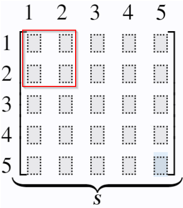
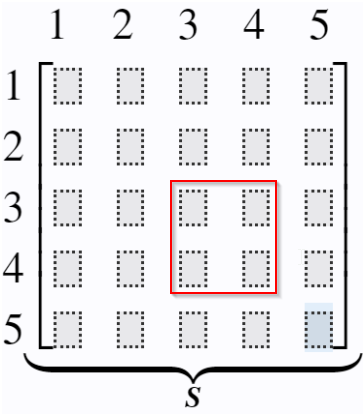
Example: Element stiffness matrix for element 3 between node 3 and 4:
1 2 3 4 5 1 2 3 4 5 [ S 33 S 34 S 43 S 44 ] ⏟ S \begin{array}{l}
\;\;\;\;\begin{array}{ccccc}
\;1 & \;2 & \;\;3 & \;\;\;4 & \;\;5
\end{array}\\
\begin{array}{c}
1\\
2\\
3\\
4\\
5
\end{array}\underset{\mathit{\mathbf{S}}}{\underbrace{\left\lbrack \begin{array}{ccccc}
& & & & \\
& & & & \\
& & S_{33} & S_{34} & \\
& & S_{43} & S_{44} & \\
& & & &
\end{array}\right\rbrack } }
\end{array} 1 2 3 4 5 1 2 3 4 5 S ⎣ ⎡ S 33 S 43 S 34 S 44 ⎦ ⎤ S 33 = ∫ x 3 x 4 d φ 3 d x d φ 3 d x d x S 34 = ∫ x 3 x 4 d φ 3 d x d φ 4 d x d x S 43 = ∫ x 3 x 4 d φ 4 d x d φ 3 d x d x S 44 = ∫ x 3 x 4 d φ 4 d x d φ 4 d x d x
\def\arraystretch{2.5}
\begin{array}{l}
S_{33} =\int_{x_3 }^{x_4 } \dfrac{d\;\varphi_3 }{d\;x}\;\dfrac{d\;\varphi_3 }{d\;x}\;d\;x\\
S_{34} =\int_{x_3 }^{x_4 } \dfrac{d\;\varphi_3 }{d\;x}\;\dfrac{d\;\varphi_4 }{d\;x}\;d\;x\\
S_{43} =\int_{x_3 }^{x_4 } \dfrac{d\;\varphi_4 }{d\;x}\;\dfrac{d\;\varphi_3 }{d\;x}\;d\;x\\
S_{44} =\int_{x_3 }^{x_4 } \dfrac{d\;\varphi_4 }{d\;x}\;\dfrac{d\;\varphi_4 }{d\;x}\;d\;x
\end{array}
S 33 = ∫ x 3 x 4 d x d φ 3 d x d φ 3 d x S 34 = ∫ x 3 x 4 d x d φ 3 d x d φ 4 d x S 43 = ∫ x 3 x 4 d x d φ 4 d x d φ 3 d x S 44 = ∫ x 3 x 4 d x d φ 4 d x d φ 4 d x We can use local node numbering to simplify things:
Now, for each element e e e x 1 x_1 x 1 x 2 x_2 x 2 φ \varphi φ d φ d x \frac{d\;\varphi }{d\;x} d x d φ S e {\mathit{\mathbf{S}}}^e S e f e {\mathit{\mathbf{f}}}^e f e
Element stiffness matrix
S e = ∫ x 1 x 2 d φ T d x d φ d x d x {\mathit{\mathbf{S}}}^e =\int_{x_1 }^{x_2 } \dfrac{d\;\varphi^T }{d\;x}\dfrac{d\;\varphi }{d\;x}\;d\;x S e = ∫ x 1 x 2 d x d φ T d x d φ d x or
S e = [ ∫ x 1 x 2 d φ 1 d x d φ 1 d x d x ∫ x 1 x 2 d φ 1 d x d φ 2 d x d x ∫ x 1 x 2 d φ 2 d x d φ 1 d x d x ∫ x 1 x 2 d φ 2 d x d φ 2 d x d x ]
\def\arraystretch{2.5}
{\mathit{\mathbf{S}}}^e =\left\lbrack \begin{array}{cc}
\int_{x_1 }^{x_2 } \dfrac{d\;\varphi_1 }{d\;x}\dfrac{d\;\varphi_1 }{d\;x}\;d\;x & \int_{x_1 }^{x_2 } \dfrac{d\;\varphi_1 }{d\;x}\dfrac{d\;\varphi_2 }{d\;x}\;d\;x\\
\int_{x_1 }^{x_2 } \dfrac{d\;\varphi_2 }{d\;x}\dfrac{d\;\varphi_1 }{d\;x}\;d\;x & \int_{x_1 }^{x_2 } \dfrac{d\;\varphi_2 }{d\;x}\dfrac{d\;\varphi_2 }{d\;x}\;d\;x
\end{array}\right\rbrack
S e = ⎣ ⎡ ∫ x 1 x 2 d x d φ 1 d x d φ 1 d x ∫ x 1 x 2 d x d φ 2 d x d φ 1 d x ∫ x 1 x 2 d x d φ 1 d x d φ 2 d x ∫ x 1 x 2 d x d φ 2 d x d φ 2 d x ⎦ ⎤ and element load vector
f e = ∫ x 1 x 2 φ T f d x {\mathit{\mathbf{f}}}^e =\int_{x_1 }^{x_2 } \varphi^T f\;d\;x f e = ∫ x 1 x 2 φ T f d x or
f e = [ ∫ x 1 x 2 f φ 1 dx ∫ x 1 x 2 f φ 2 dx ]
\def\arraystretch{2.0}
{\mathit{\mathbf{f}}}^e =\left\lbrack \begin{array}{c}
\int_{x_1 }^{x_2 } f\varphi_1 \;\textrm{dx}\\
\int_{x_1 }^{x_2 } f\varphi_2 \;\textrm{dx}
\end{array}\right\rbrack
f e = ⎣ ⎡ ∫ x 1 x 2 f φ 1 dx ∫ x 1 x 2 f φ 2 dx ⎦ ⎤ For each element e e e S e {\mathit{\mathbf{S}}}^e S e f e {\mathit{\mathbf{f}}}^e f e S \mathit{\mathbf{S}} S f \mathit{\mathbf{f}} f
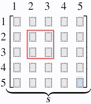
Element 1: S([1,2],[1,2])
Element 2: S([2,3],[2,3])
Element 3: S([3,4],[3,4])
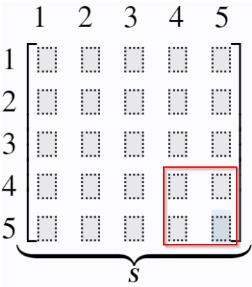
Element 4: S([4,5],[4,5])
We need to add each element contribution to the global stiffness matrix.
S ii new = S ii old + S 11 e S ij new = S ij old + S 12 e ⋮ \begin{array}{l}
S_{\textrm{ii}}^{\textrm{new}} =S_{\textrm{ii}}^{\textrm{old}} +S_{11}^e \\
S_{\textrm{ij}}^{\textrm{new}} =S_{\textrm{ij}}^{\textrm{old}} +S_{12}^e \\
\vdots
\end{array} S ii new = S ii old + S 11 e S ij new = S ij old + S 12 e ⋮ f i new = f i old + f 1 e f j new = f j old + f 2 e \begin{array}{l}
f_i^{\textrm{new}} =f_i^{\textrm{old}} +f_1^e \\
f_j^{\textrm{new}} =f_j^{\textrm{old}} +f_2^e
\end{array} f i new = f i old + f 1 e f j new = f j old + f 2 e or on matrix form
S ( row , col ) S(\text{row},\text{col}) S ( row , col ) where row denotes the array containing the row indices and col the column indices. Thus we could write
S ( [ i , j ] , [ i , j ] ) S([i,j],[i,j]) S ([ i , j ] , [ i , j ]) to mean a sub-matrix of S S S i i i j j j i i i j j j
The corresponding Matlab (or Julia) syntax is
S([i ,j ],[i ,j ]) = S([i ,j ],[i ,j ]) + SeAll nodes that have several elements will get contributions from each element. We are "accumulating" stiffness to these nodes from the elements.
Contribution from element 1
S ( [ 1 , 2 ] , [ 1 , 2 ] ) 2 × 2 = S ( [ 1 , 2 ] , [ 1 , 2 ] ) 2 × 2 + S 2 × 2 e 1 {\mathit{\mathbf{S}}\left(\left\lbrack 1,2\right\rbrack ,\left\lbrack 1,2\right\rbrack \right)}_{2\times 2} ={\mathit{\mathbf{S}}\left(\left\lbrack 1,2\right\rbrack ,\left\lbrack 1,2\right\rbrack \right)}_{2\times 2} +S_{2\times 2}^{e_1 } S ( [ 1 , 2 ] , [ 1 , 2 ] ) 2 × 2 = S ( [ 1 , 2 ] , [ 1 , 2 ] ) 2 × 2 + S 2 × 2 e 1 1 2 3 4 5 1 2 3 4 5 [ S 11 1 S 12 1 S 21 1 S 22 1 ] \begin{array}{l}
\;\;\;\;\begin{array}{ccccc}
\;\;\;\;\;1 & \;\;\;2 & 3 & 4 & 5
\end{array}\\
\begin{array}{c}
1\\
2\\
3\\
4\\
5
\end{array}\left\lbrack \begin{array}{ccccc}
S_{11}^1 & S_{12}^1 & & & \\
S_{21}^1 & S_{22}^1 & & & \\
& & & & \\
& & & & \\
& & & &
\end{array}\right\rbrack
\end{array} 1 2 3 4 5 1 2 3 4 5 ⎣ ⎡ S 11 1 S 21 1 S 12 1 S 22 1 ⎦ ⎤ Contribution from element 2
S ( [ 2 , 3 ] , [ 2 , 3 ] ) 2 × 2 = S ( [ 2 , 3 ] , [ 2 , 3 ] ) 2 × 2 + S e 2 {\mathit{\mathbf{S}}\left(\left\lbrack 2,3\right\rbrack ,\left\lbrack 2,3\right\rbrack \right)}_{2\times 2} ={\mathit{\mathbf{S}}\left(\left\lbrack 2,3\right\rbrack ,\left\lbrack 2,3\right\rbrack \right)}_{2\times 2} +S_{\;}^{e_2 } S ( [ 2 , 3 ] , [ 2 , 3 ] ) 2 × 2 = S ( [ 2 , 3 ] , [ 2 , 3 ] ) 2 × 2 + S e 2 1 2 3 4 5 1 2 3 4 5 [ S 11 1 S 12 1 S 21 1 S 22 1 + S 11 2 S 12 2 S 21 2 S 22 2 ] \begin{array}{l}
\;\;\;\;\begin{array}{ccccc}
\;\;\;\;\;1 & \;\;\;\;\;\;\;\;2 & \;\;\;\;\;\;\;\;3 & 4 & 5
\end{array}\\
\begin{array}{c}
1\\
2\\
3\\
4\\
5
\end{array}\left\lbrack \begin{array}{ccccc}
S_{11}^1 & S_{12}^1 & & & \\
S_{21}^1 & S_{22}^1 +S_{11}^2 & S_{12}^2 & & \\
& S_{21}^2 & S_{22}^2 & & \\
& & & & \\
& & & &
\end{array}\right\rbrack
\end{array} 1 2 3 4 5 1 2 3 4 5 ⎣ ⎡ S 11 1 S 21 1 S 12 1 S 22 1 + S 11 2 S 21 2 S 12 2 S 22 2 ⎦ ⎤ etc
Since u 1 u_1 u 1
We also need to modify the right-hand side, since u 1 u_1 \; u 1
f new = f old + g − [ S 11 S 21 ⋮ S 51 ] u 1 {\mathit{\mathbf{f}}}^{\textrm{new}} ={\mathit{\mathbf{f}}}^{\textrm{old}} +\mathit{\mathbf{g}}-\left\lbrack \begin{array}{c}
S_{11} \\
S_{21} \\
\vdots \\
S_{51}
\end{array}\right\rbrack u_1 f new = f old + g − ⎣ ⎡ S 11 S 21 ⋮ S 51 ⎦ ⎤ u 1 and finally our equation system is
[ S 22 S 23 S 24 S 25 S 32 ⋮ S 42 ⋮ S 52 ⋯ ⋯ S 55 ] [ u 2 u 3 u 4 u 5 ] = [ f 2 + 0 − S 21 u 1 f 3 + 0 − S 31 u 1 f 4 + 0 − S 41 u 1 f 5 − 1 ⏟ g 5 − S 51 u 1 ] \left\lbrack \begin{array}{cccc}
S_{22} & S_{23} & S_{24} & S_{25} \\
S_{32} & & & \vdots \\
S_{42} & & & \vdots \\
S_{52} & \cdots & \cdots & S_{55}
\end{array}\right\rbrack \left\lbrack \begin{array}{c}
u_2 \\
u_3 \\
u_4 \\
u_5
\end{array}\right\rbrack =\left\lbrack \begin{array}{c}
f_2 +0-S_{21} u_1 \\
f_3 +0-S_{31} u_1 \\
f_4 +0-S_{41} u_1 \\
f_{5}\underset{g_{5}}{\underbrace{-1}}-S_{51}u_{1}
\end{array}\right\rbrack ⎣ ⎡ S 22 S 32 S 42 S 52 S 23 ⋯ S 24 ⋯ S 25 ⋮ ⋮ S 55 ⎦ ⎤ ⎣ ⎡ u 2 u 3 u 4 u 5 ⎦ ⎤ = ⎣ ⎡ f 2 + 0 − S 21 u 1 f 3 + 0 − S 31 u 1 f 4 + 0 − S 41 u 1 f 5 g 5 − 1 − S 51 u 1 ⎦ ⎤ { − d 2 u d x 2 = 1 for x ∈ [ 1 3 ] u ( 1 ) = 2 d u d x ( 3 ) = − 1
\def\arraystretch{2.0}
\left\lbrace \begin{array}{ll}
-\dfrac{d^2 u}{d x^2}=1 & \textrm{for}\;x\in \left\lbrack 1\;3\right\rbrack \\
u\left(1\right)=2 & \\
\dfrac{d\;u}{d\;x}\left(3\right)=-1 &
\end{array}\right.
⎩ ⎨ ⎧ − d x 2 d 2 u = 1 u ( 1 ) = 2 d x d u ( 3 ) = − 1 for x ∈ [ 1 3 ] clear
a = 1 ; b = 3 ;
N = 4 ;
xnod = linspace (a,b,N+1 );
nodes = [(1 :N)',(2 :N+1 )'];
syms x
Phi = @(x1,x2,x)[(x-x2)/(x1-x2), -(x-x1)/(x1-x2)];
Dphi = matlabFunction(diff(Phi,x));
neq = N+1 ;
S = zeros (neq,neq); F = zeros (neq,1 );
for iel = 1 :N
inods = nodes(iel,:);
x1 = xnod(inods(1 ));
x2 = xnod(inods(2 ));
phi = Phi(x1,x2,x);
dphi = Dphi(x1,x2);
Se = double(int(dphi.'*dphi,x,x1,x2));
fe = double(int(1 *phi.',x,x1,x2));
S(inods,inods) = S(inods,inods) + Se;
F(inods) = F(inods) + fe;
end
presc = 1 ;
alldofs = 1 :N+1 ;
free = setdiff(alldofs,presc);
u = zeros (neq,1 ); u(presc) = 2 ;
g = zeros (neq,1 );
g(1 ) = -0 ;
g(end ) = -1 ;
F = F+g-S(:,presc)*u(presc);
u(free) = S(free,free)\F(free) Show output
u = 5 x1
2.0000
2.3750
2.5000
2.3750
2.0000
syms ue(x)
DE = -diff(ue,x,2 ) == 1 ;
du = diff(ue,x,1 );
BC = [ue(1 )==2 , du(3 )==-1 ];
ue = dsolve(DE,BC)1 2 − x ( x − 4 ) 2 \dfrac{1}{2}-\dfrac{x\,{\left(x-4\right)} }{2} 2 1 − 2 x ( x − 4 ) Plot the solution
figure
fplot(ue, [1 ,3 ],'r' ,'DisplayName' ,'Exact solution' ); hold on
plot (xnod,u,'ob-' ,'DisplayName' ,'Approximation' )
legend show
1: Approximate solution using 4 linear elements
L 2 err : = ∫ 1 3 ( U − u e ) 2 d x L_2 \textrm{err}:=\sqrt{\int_1^3 {\left(U-u_e \right)}^2 \;d\;x} L 2 err := ∫ 1 3 ( U − u e ) 2 d x For each element e e e i i i j j j
U ( x ) = φ ( x ) ⋅ u e
U(x) = \boldsymbol \varphi(x) \cdot \boldsymbol u_e
U ( x ) = φ ( x ) ⋅ u e Specifically for our case we have
U ( x ) = [ φ i , φ j ] ⋅ [ u i , u j ] U(x) = [\varphi_i,\ \varphi_j] \cdot [u_i,\ u_j] U ( x ) = [ φ i , φ j ] ⋅ [ u i , u j ] L2err = 0 ;
for iel = 1 :N
inods = nodes(iel,:);
x1 = xnod(inods(1 ));
x2 = xnod(inods(2 ));
phi = Phi(x1,x2,x);
U = phi*u(inods);
L2err = L2err + int((U-ue)^2 ,x,x1,x2);
end
L2err = double(sqrt (L2err))