ElasticitySolverTraction

Table of contents

2D Static Linear Elasticity - linear triangles
Solution strategy
Creating the geometry
Preliminaries
Create the mesh
Material model
Compute the stiffness matrix
Traction load
Essential boundary conditions
Live lecture

2D Static Linear Elasticity - linear triangles

Solve the static linear elasticity PDE using linear triangle elements and an external traction force.

\left\lbrace \begin{array}{ll} -\nabla \cdot \bm \sigma = \bm f & \textrm{in }\Omega \\ \bm \sigma =2\mu \bm \varepsilon + \lambda \textrm{tr} \bm \varepsilon \bm I & \textrm{in } \Omega \\ \bm \sigma \cdot \bm n = \bm F & \textrm{on}\;E_2 \\ \bm u_y =0 & \textrm{on}\;E_1 \\ \bm u_x =0 & \textrm{on}\;E_4 \end{array}\right.

Let $E=2200\textrm{MPa},$ $\nu =0\ldotp 33$ , $t=1\;\textrm{mm}$ , use plane stress and implement a solver to numerically find the displacement field and compute the stress field.

Solution strategy

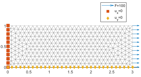
Create a simple geometry that is verifiable by hand. In this case we will create a rectangle on which we can apply the load case shown in the figure above. We want to apply boundary conditions such that the rectangle is in pure tension, meaning we only have stress in the x-direction. All other stress i zero. Thus we can compute the displacement analytically:

\delta =\dfrac{F\;L}{E\;A}\;\textrm{and}\;\sigma_x =\dfrac{F}{A}

where $A=1\cdot {t\;\textrm{mm} }^2$ and $L=3\;\textrm{mm}$ .

Creating the geometry

This assumes you have access to the PDE toolbox in matlab. Check this by running ver. Otherwise you need to install that toolbox.

clear
model = createpde;
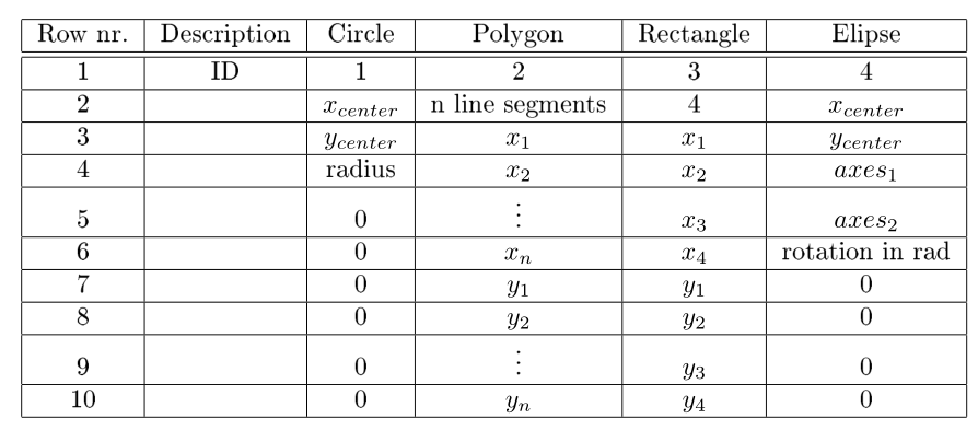
R1 = [3,4,0,3,3,0,0,0,1,1]'; %Create a rectangle
gd = [R1];
sf = 'R1'; % What boolean operation are we running?
ns = char('R1')'; % Label the geometric entities, so we know which is which.
g = decsg(gd,sf,ns);
geometryFromEdges(model,g);
figure
pdegplot(model,'EdgeLabels','on')
title('Imported geometry with regions')

Preliminaries

Weak form: Find the displacement field $\bm u$ , with $\bm u = \bm g$ on the boundary $\partial \Omega_D$ , such that

\int_{\Omega } \bm \sigma \left(\bm u\right):\bm \varepsilon \left(\bm v\right)\;d\Omega =\int_{\Omega } \bm f\cdot \bm v\;d\Omega +\int_{\partial \Omega } \bm F \cdot \bm v ds \quad \forall v\;\textrm{that}\;\textrm{are}\;0\;\textrm{on}\;\partial \Omega_D \;\;\;\;\;\left(1\right)

We have (using the Mandel notation), the element stiffness matrix

\bm S_K =\int_K \left(2\mu {\mathit{\mathbf{B} } }_{\varepsilon }^T {\mathit{\mathbf{B} } }_{\varepsilon } +\lambda {\mathit{\mathbf{B} } }_D {\mathit{\mathbf{B} } }_D \right)d\;K

the element load vector (zero in our problem)

\bm f_K =\int_K \bm \Phi^T \bm f \left(\bm x\right) dK

the traction (external force) vector

\bm g_E =\int_E \bm \Phi_E^T \bm t \left(\bm x\right) dE

where $E$ denotes edge (in 2D, where as in 3D it would be a surface). The edge element is one spatial dimension lower, we are formulating the equations on an edge instead of a triangle. For the edge element we have

\bm \Phi_E \overset{2D\;\textrm{lin} }{=} \left\lbrack \begin{array}{cccc} \varphi_1^E & 0 & \varphi_2^E & 0\\ 0 & \varphi_1^E & 0 & \varphi_2^E \end{array}\right\rbrack , \quad \bm \varphi^E \overset{2D\;\textrm{lin} }{=} \left\lbrack \begin{array}{cc} 1+\xi & \xi \end{array}\right\rbrack

\bm B_{\varepsilon } :=\left\lbrack \begin{array}{ccccc} \dfrac{\partial \varphi_1 }{\partial x} & 0 & \dfrac{\partial \varphi_2 }{\partial x} & 0 & \cdots \\ 0 & \dfrac{\partial \varphi_1 }{\partial y} & 0 & \dfrac{\partial \varphi_2 }{\partial y} & \cdots \\ \dfrac{1}{\sqrt{2} }\dfrac{\partial \varphi_1 }{\partial y} & \dfrac{1}{\sqrt{2} }\dfrac{\partial \varphi_1 }{\partial x} & \dfrac{1}{\sqrt{2} }\dfrac{\partial \varphi_2 }{\partial y} & \dfrac{1}{\sqrt{2} }\dfrac{\partial \varphi_2 }{\partial x} & \cdots \end{array}\right\rbrack

\bm B_{\textrm{div} } :=\left\lbrack \begin{array}{ccccc} \dfrac{\partial \varphi_{\;1} }{\partial x} & \dfrac{\partial \varphi_{\;1} }{\partial y} & \dfrac{\partial \varphi_{\;2} }{\partial x} & \dfrac{\partial \varphi_{\;2} }{\partial y} & \cdots \end{array}\right\rbrack

\bm u_K \left(\bm x \right)\approx \bm U_K \left(\bm x \right)={\underset{\Phi_K \left(\bm x \right)}{\underbrace{\left\lbrack \begin{array}{cccccc} \varphi_1 \left(\bm x \right) & 0 & \varphi_2 \left(\bm x \right) & 0 & \varphi_3 \left(\bm x \right) & 0\\ 0 & \varphi_1 \left(\bm x \right) & 0 & \varphi_2 \left(\bm x \right) & 0 & \varphi_3 \left(\bm x \right) \end{array}\right\rbrack } } }_{2\textrm{x6} } {\left\lbrack \begin{array}{c} u_x^1 \\ u_y^1 \\ u_x^2 \\ u_y^2 \\ u_x^3 \\ u_y^3 \end{array}\right\rbrack }_{6\textrm{x1} }

Tasks:

Create mesh
Compute the stiffness matrix
Compute the traction load
Solve the linear system $\mathit{\mathbf{S} }\;\mathit{\mathbf{u} }=\mathit{\mathbf{f} }$
Compare displacement error
Compute the stress

Create the mesh

% Start with the mesh
h = 5 %mm

h = 5

mesh = generateMesh(model, 'Hmax', h, 'Hmin', h/2,...
    'hgrad',1.99, 'GeometricOrder', 'linear');
% pdemesh(mesh)

P = mesh.Nodes';
nodes = mesh.Elements';

% Visualize the mesh
figure; hold on
patch('Vertices', P, 'Faces', nodes,'FaceColor', 'c', ...
    'EdgeAlpha',0.3)
axis equal tight

plot(P(:,1),P(:,2),'ok','MarkerFaceColor','k','MarkerSize',10)
text(P(:,1)-0.03,P(:,2),cellstr(num2str([1:size(P,1)]')), ...
    'Color','w','FontSize',6)
for iel = 1:size(nodes,1)
    inod = nodes(iel,:);
    xm = mean(P(inod,1));
    ym = mean(P(inod,2));
    text(xm,ym,num2str(iel),'FontSize',6)
end

[nele, knod] = size(nodes);
[nnod, dof] = size(P);
neq = nnod*dof;

phi = @(xi,eta)[1-xi-eta, xi, eta];
Bh = [-1,1,0
      -1,0,1];

Material model

E = 2200; %MPa
nu = 0.33;
t = 1; %mm

%Plane Stress
lambda = E*nu/(1-nu^2);
mu = E/(2*(1+nu));

Compute the stiffness matrix

\bm S_K =\int_K \left(2\mu {\mathit{\mathbf{B} } }_{\varepsilon }^T {\mathit{\mathbf{B} } }_{\varepsilon } +\lambda {\mathit{\mathbf{B} } }_D {\mathit{\mathbf{B} } }_D \right)d\;K

\bm B_{\varepsilon } :=\left\lbrack \begin{array}{ccccc} \dfrac{\partial \varphi_1 }{\partial x} & 0 & \dfrac{\partial \varphi_2 }{\partial x} & 0 & \cdots \\ 0 & \dfrac{\partial \varphi_1 }{\partial y} & 0 & \dfrac{\partial \varphi_2 }{\partial y} & \cdots \\ \dfrac{1}{\sqrt{2} }\dfrac{\partial \varphi_1 }{\partial y} & \dfrac{1}{\sqrt{2} }\dfrac{\partial \varphi_1 }{\partial x} & \dfrac{1}{\sqrt{2} }\dfrac{\partial \varphi_2 }{\partial y} & \dfrac{1}{\sqrt{2} }\dfrac{\partial \varphi_2 }{\partial x} & \cdots \end{array}\right\rbrack

\bm B_{\textrm{div} } :=\left\lbrack \begin{array}{ccccc} \dfrac{\partial \varphi_{\;1} }{\partial x} & \dfrac{\partial \varphi_{\;1} }{\partial y} & \dfrac{\partial \varphi_{\;2} }{\partial x} & \dfrac{\partial \varphi_{\;2} }{\partial y} & \cdots \end{array}\right\rbrack

% Pre-allocate 
S = zeros(neq,neq);
sq = 1/sqrt(2);
for iel = 1:nele
    inod = nodes(iel,:);
    iP = P(inod,:);
    
    locdof = zeros(1,6);
    locdof(1:2:end) = inod*2-1;
    locdof(2:2:end) = inod*2;

    J = Bh*iP;
    area = det(J) * 1/2;

    B = J\Bh;

    Beps = zeros(3,6);
    Beps(1,1:2:end) = B(1,:);
    Beps(2,2:2:end) = B(2,:);
    Beps(3,1:2:end) = sq*B(2,:);
    Beps(3,2:2:end) = sq*B(1,:);

    Bdiv = zeros(1,6);
    Bdiv(1:2:end) = B(1,:);
    Bdiv(2:2:end) = B(2,:);

    Se = t*(2*mu*Beps'*Beps + lambda*Bdiv'*Bdiv)*area;

    S(locdof, locdof) = S(locdof, locdof) + Se;
end

% figure
% spy(S)

Traction load

%Region
E2 = findNodes(mesh,'region','Edge',2);
%load
fload = [100,0]';

phi=@(xi)[1-xi,xi];

eleInds = find(sum(ismember(nodes,E2),2)>1);

F = zeros(neq,1);
ieqs = zeros(2*2,1);
PHI = zeros(2,4);
L = 0;
nele = length(eleInds);
for iel = 1:nele
    indTri = eleInds(iel);
    iTri = nodes(indTri,:);
    iEdgeNodes = iTri(ismember(iTri,E2));

    ieqs(1:2:end) = 2*iEdgeNodes-1; %x-dofs
    ieqs(2:2:end) = 2*iEdgeNodes-0; %y-dofs
    xc = P(iEdgeNodes,:);
    h = norm(xc(end,:)-xc(1,:));
    L = L + h;

    xi = 0.5; iw = 1;
    PHI(1,1:2:end) = phi(xi);
    PHI(2,2:2:end) = phi(xi);

    fe = PHI'*fload(:)*t*h*iw;

    F(ieqs) = F(ieqs) + fe;
end

F = F/(L*t);

Verify the traction load

sum(F(1:2:end))

ans = 100

Visualize the load vector

figure; hold on
patch('Vertices', P, 'Faces', nodes,'FaceColor', 'c', ...
    'EdgeAlpha',0.1,'DisplayName','linear mesh')
axis equal tight

quiver(P(E2,1), P(E2,2), F(E2*2-1), F(E2*2-0),'b', ...
    'DisplayName','F=[100,0]N');

Essential boundary conditions

u = zeros(neq,1);

Edge 1

E1 = findNodes(mesh,'region','Edge',1);
% Prescribe displacements
u(E1*2) = 0; %y-displacements
plot(P(E1,1),P(E1,2),'bd','MarkerFaceColor','b','Displayname','u_y=0')

Edge 4

E4 = findNodes(mesh,'region','Edge',4);
% prescribed displacement
u(E4*2-1) = 0; %x-displacements
plot(P(E4,1),P(E4,2),'rs','MarkerFaceColor','r','Displayname','u_x=0')

hl = legend('show'); 
set(hl,'Position',[0.60 0.69 0.20 0.20]);

Modify the right-hand side

\mathbf{S}\;\mathbf{u}=\mathbf{f}-{\mathbf{S} }_{\mathbf{p} } \;{\mathbf{u} }_{\mathbf{p} }

presc = unique([E4*2-1, E1*2]);
free = setdiff(1:neq,presc);

F = F - - S(:,presc)*u(presc);

Solve the linear system

u(free) = S(free,free)\F(free);

Visualize the displacement field

U = [u(1:2:end), u(2:2:end)];
UR = sum(U.^2,2).^0.5;
scale = 3;
figure; hold on
pdegplot(model,'EdgeLabels','off')
patch('Vertices', P+U*scale, 'Faces', nodes,'FaceColor', 'interp', ...
    'EdgeAlpha',0.1,'CData',UR)
axis equal tight
title(['Displacement field, scale: ',num2str(scale)])

Verification

A=1*t; L = 3; f = 100;
deltax = f*L/(E*A)

deltax = 0.1364

deltay = -nu*(deltax/L)*1

deltay = -0.0150

ux = U(E2,1)

ux = 2x1    
    0.1364
    0.1364

uy = U(findNodes(mesh,'region','Edge',3),2)

uy = 2x1    
   -0.0150
   -0.0150