Table of contents
We create a model of a beam by aligning a uniform beam with the \(x\)-axis in the \(xy\)-plane with a translational degree of freedom only in the \(y\)-direction and such that the beam can bend about the \(z\)-axis, out of plane. Thus we have two degrees of freedom, rotation about the \(z\) axis, \(\theta_{z}\) and translation (of deflection) in the \(y\)-axis, \(u_{y}\). This corresponds to the elementary beam theory, or engineering beam theory also known as Euler-Bernoulli beam theory. There are beam models that also allow the beam to stretch as well as bend by adding \(u_{x}\) to the degrees of freedom which also includes non-zero shear strain \(\gamma_{xz}\), one such theory is the Timoshenko beam theory see e.g., [1] and [2] which are typically used for beams which are significantly higher. Although, as we shall see, the Euler-Bernoulli theory involves many assumptions and simplifications, it provides accurate predictions for many important practical engineering problems.
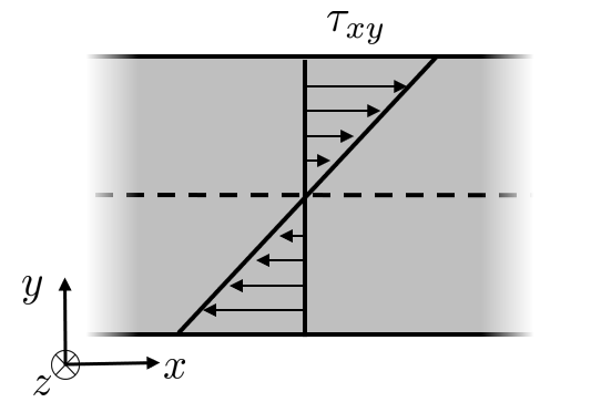
Consider beam a cross section of a beam normal to the \(x\)-axis, we have (due to symmetry and load in the \(xy\) plane) the only non-zero stress components \(\sigma_{xx}\) and \(\tau_{xy}\) see Figure 1
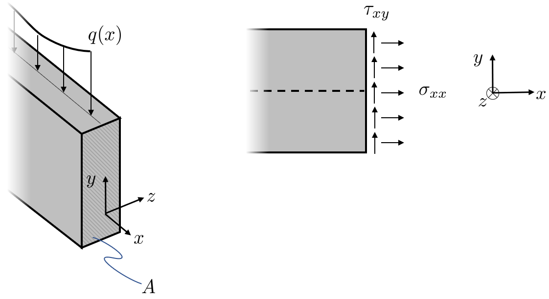
From Figure 1 we can formulate equilibrium equations, beginning with the normal force which is assumed to be static such that the resultant is zero
\[ N=\int_{A}\sigma_{xx}dy dz=0 \]Furthermore these stress components give rise to a bending moment \(M\) and a vertical shear force \(T\) according to the figures above
\[ M=\int_{A}y\sigma_{xx}dy dz,\quad T=\int_{A}\tau_{xy}dy dz \]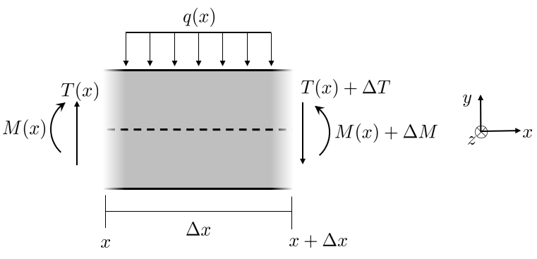
For an infinitesimal element of the beam, see Figure 2, we get an equilibrium equation in the positive \(y\)-direction
\[ \uparrow:\quad\int_{x}^{x+\Delta x}-q(x)dx+T-(T+\Delta T)=0 \]the infinitesimal element is arbitrarily small such that we can let \(\Delta x\rightarrow0\) and in the limit we get
\[ \boxed{-q(x)=\dfrac{dT}{dx}} \]The moment equilibrium yields
\[ \circlearrowleft x:\quad-M+(M+\Delta M)-(T+\Delta T)\Delta x-\int_{x}^{x+\Delta x}q(x)xdx=0 \]with \(\int_{x}^{x+\Delta x}qxdx=\frac{1}{2}q\left(\Delta x\right)^{2}\) we get
\[ \Delta M-T\Delta x-\underset{\text{small}\approx0}{\underbrace{\Delta T\Delta x}}-\frac{1}{2}q\underset{\text{small}\approx0}{\underbrace{\left(\Delta x\right)^{2}}}=0 \]Thus we get in the limit
\[ \boxed{T=\dfrac{dM}{dx}} \]This can be inserted into (4) to yield
\[ \boxed{-q(x)=\dfrac{d^{2}M}{dx^{2}}} \]The defining assumption in the Euler-Bernoulli theory dates back to Jacob Bernoulli (1654-1705) and states:
Plane sections normal to the beam axis remain plane and normal to
the beam axis during the deformation.
Let \(w(x)\) denote \(u_{y}\) and consider the deformed beam
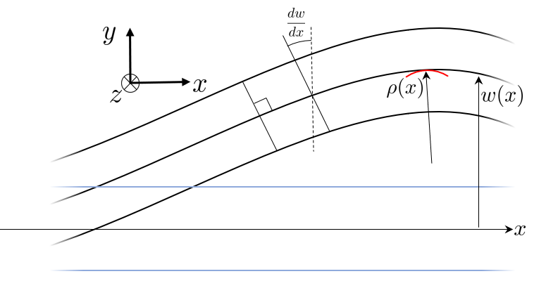
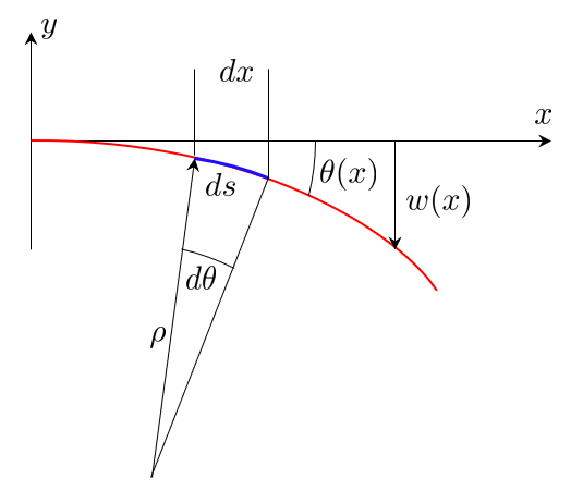
From the local beam deformation shown in Figure 3, we can define kinematic relations posed on an infinitesimal element, beginning with the segment length
\[ ds=\dfrac{dx}{\cos\theta}\approx dx \]The slope is given by
\[ \dfrac{dw}{dx}=\tan\theta\approx\theta \]furthermore, using small angle approximation, the curvature of the segment is given by
\[ ds=\rho d\theta\Rightarrow\dfrac{d\theta}{dx}\approx\dfrac{1}{\rho} \]Using the newly formed relation we get the beam curvature related to the deflection by
\[ \left.\begin{array}{c} \theta=\dfrac{dw}{dx}\\ \dfrac{d\theta}{dx}=\dfrac{1}{\rho} \end{array}\right\} \dfrac{1}{\rho}=\dfrac{d^{2}w}{dx^{2}} \]Consider the displacements local of an infinitesimal element
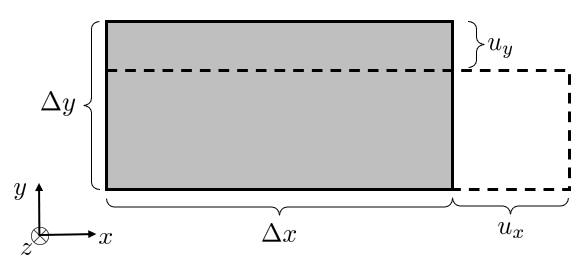
The engineering strains can be formulated by the small strain assumption
\[ \varepsilon_{xx}=\dfrac{u_{x}}{\Delta x}\rightarrow\dfrac{du_{x}}{dx} \]for the strains due to contraction we make the assumption that the displacements are so small that the resulting strains become negligible.
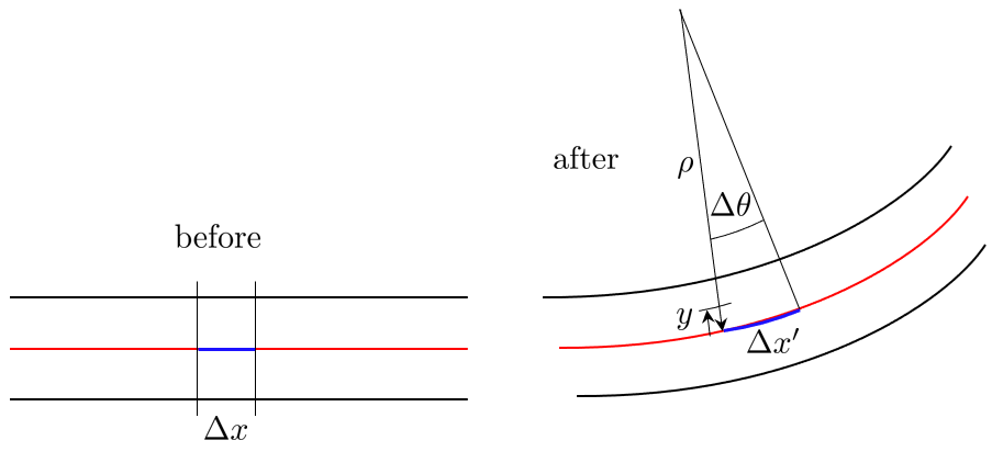
The displacement kinematics state
and using the circle segment, we can express this using the radius and angle
\[\begin{aligned} u_{x} & =(\rho-y)\Delta\theta-\rho\Delta\theta \\ & =-y\Delta\theta \end{aligned}\]and thus, using (13) and (14) , the strain becomes
\[ \varepsilon_{xx}=\dfrac{u_{x}}{\Delta x}=\dfrac{u_{x}}{\rho\Delta\theta}=-\dfrac{y}{\rho} \]combining this with the curvature relation from (12) we end up with the strain equation
\[ \boxed{\varepsilon_{xx}=-y\dfrac{d^{2}w}{dx^{2}}} \]Using Hooke's law we get
\[ \sigma_{xx}=E\varepsilon_{xx} \]which we can insert into (2) and combine with (16) to form
We note that if the elastic modulus and axial strain do not vary across the cross-sectional area (or along the \(yz-\) plane) we can simplify to
\[ M=-E\dfrac{d^{2}w}{dx^{2}}\int_{A}y^{2}dA \]We identify the integral as the moment of inertia, \(I=\int_{A}y^{2}dA\) and thus the bending moment is determined from
\[ M=-EI\dfrac{d^{2}w}{dx^{2}} \]where \(EI\) is known as the bending stiffness. It is interesting to note the relation to differential geometry where the curvature of a curve is given by
\[ \kappa=\dfrac{d^{2}w/dx^{2}}{\left[1+(dw/dx)^{2}\right]^{3/2}} \]and as the slope \(dw/dx\) is assumed to be small, we can obtain the approximation from this expression as well
\[ \kappa\approx\dfrac{d^{2}w}{dx^{2}}=\dfrac{1}{\rho}. \]The expression for the bending moment (19) is inserted into (8) and we finally arrive at the Bernoulli's beam equation
\[ \boxed{\dfrac{d^{2}}{dx}\left(EI\dfrac{d^{2}w}{dx^{2}}\right)=q} \]Note that we have from the general Hooke's law and plane stress assumption:
\[ \sigma_{xx}=\dfrac{E(1-\nu)}{(1+\nu)(1-2\nu)}\varepsilon_{xx} \]and that since earlier, the assumption was made that all strains but \(\varepsilon_{xx}\) are zero and thus \(\tau_{xy}=\tau_{xz}=\tau_{yz}=0\) due to e.g., \(\tau_{xy}=G\gamma_{xy}=0\) which is in contradiction because the shear force is non-zero
\[ T=\int_{A}\tau_{xy}dA\neq0 \]This inconsistency stems from the fact that we try to simplify a three dimensional problem into a simpler form. We need to neglect plane stress and just utilize the 1D form of Hooke's law:
\[ \sigma_{xx}=E\varepsilon_{xx} \]and accept the contradiction \(\sigma_{xy}\neq0\) and \(\gamma_{xy}=0\). Although Bernoulli's beam theory presented above involves many assumptions and simplifications, it provides a good accuracy to a variety of engineering problems of practical importance. For beams with high aspect ratios, i.e., \(\text{length}>>[\text{hight},\text{width}]\), the theory is satisfactory, and for higher beams, one can utilize e.g., the Timoshenko theory or stick to general plane stress theory.
We start with
\[ \dfrac{d^{2}M}{dx^{2}}+q=0,\quad\text{for }x\in[a,b] \]Multiply by \(v\) and integrate by parts
\[ \int_{a}^{b}\left(\dfrac{d^{2}M}{dx^{2}}+q\right)vdx=0 \] \[ -\int_{a}^{b}\dfrac{dv}{dx}\dfrac{dM}{dx}dx+\left[\dfrac{dM}{dx}v\right]_{a}^{b}+\int_{a}^{b}qvdx=0 \]integrate the left term by parts once more
\[ \int_{a}^{b}\dfrac{d^{2}v}{dx^{2}}Mdx-\left[M\dfrac{dv}{dx}\right]_{a}^{b}+\left[\underset{T=\frac{dM}{dx}}{\underbrace{T}}v\right]_{a}^{b}+\int_{a}^{b}qvdx=0 \]such that we finally arrive at the weak form of the Bernoulli beam equation
\[ \boxed{\int_{a}^{b}\dfrac{d^{2}v}{dx^{2}}EI\dfrac{d^{2}w}{dx^{2}}dx=\int_{a}^{b}qvdx+\left[M\dfrac{dv}{dx}\right]_{a}^{b}+\left[Tv\right]_{a}^{b}} \]Notice that the weak form provides us with two Neumann (or natural) boundary conditions (also known as static boundary conditions) where the shear force \(T\) and/or bending moment \(M\) is known at \(a\) and/or \(b\). The natural boundary conditions along with the essential (Dirichlet) boundary conditions (also known as kinematic boundary conditions), where \(w\) and/or \(\theta\) (or \(dw/dx\)) is known at \(a\) and/or \(b\), enable us to model any case for the beam.


Approximate the solution by
\[ w(x)\approx\sum_{i=1}^{n}\varphi_{i}(x)u_{i} \]and let \(\bm{\varphi}=[\varphi_{1},\varphi_{2},...,\varphi_{n}]\), \({\bf u}=[u_{1},u_{2},...,u_{n}]^{T}\) then we can write
\[ \dfrac{d^{2}w}{dx^{2}}\approx{\bf B}{\bf u},\quad{\bf B}=\dfrac{d^{2}\bm{\varphi}}{dx^{2}}=\left[\dfrac{d^{2}\varphi_{1}}{dx^{2}},\dfrac{d^{2}\varphi_{n}}{dx^{2}},...,\dfrac{d^{2}\varphi_{n}}{dx^{2}}\right] \]and let \(\bm{\varphi}=[\varphi_{1},\varphi_{2},...,\varphi_{n}]\), \({\bf u}=[u_{1},u_{2},...,u_{n}]^{T}\) then we can write
\[ \dfrac{d^{2}w}{dx^{2}}\approx{\bf B}{\bf u},\quad{\bf B}=\dfrac{d^{2}\bm{\varphi}}{dx^{2}}=\left[\dfrac{d^{2}\varphi_{1}}{dx^{2}},\dfrac{d^{2}\varphi_{n}}{dx^{2}},...,\dfrac{d^{2}\varphi_{n}}{dx^{2}}\right] \]we insert the approximation into the weak form in (30) and use Galerkin's method to set \(v=\varphi_{i}\), \(\frac{dv}{dx}=\frac{d\varphi_{i}}{dx}\) and \(\frac{d^{2}v}{dx^{2}}=\frac{d^{2}\varphi_{i}}{dx^{2}}\) to get
\[ \left(\int_{a}^{b}{\bf B}^{T}EI{\bf B}dx\right){\bf u}=\int_{a}^{b}\bm{\varphi}^{T}qdx-\left[\dfrac{d\bm{\varphi}}{dx}^{T}M\right]_{a}^{b}+\left[\bm{\varphi}^{T}T\right]_{a}^{b} \]from which we identify the matrices
where \({\bf S}\) is the stiffness matrix, \({\bf f}_{L}\) the load vector and \({\bf f}_{B}\) the boundary vector. Thus we end up with the linear system
\[ {\bf S}{\bf u}={\bf f} \]with \({\bf f}={\bf f}_{L}+{\bf f}_{B}\).
Now we consider just one element from \(x_{1}\) to \(x_{2}\) where we have
\[ w(x)=\bm{\varphi}_{e}{\bf u}_{e} \]and
\[ {\bf S}_{e}{\bf u}_{e}={\bf f}_{e}={\bf f}_{Le}+{\bf f}_{Be} \]where
\[\begin{aligned} & {\bf S}_{e} =\int_{x_{1}}^{x_{2}}{\bf B}_{e}^{T}EI{\bf B}_{e}dx \\ & {\bf f}_{Le} =\int_{x_{1}}^{x_{2}}\bm{\varphi}_{e}^{T}qdx \\ & {\bf f}_{Be} =\left[\bm{\varphi}_{e}^{T}T\right]_{x_{1}}^{x_{2}}-\left[\dfrac{d\bm{\varphi}_{e}}{dx}^{T}M\right]_{x_{1}}^{x_{2}} \end{aligned}\]Inside the beam element, i.e., away from the boundaries such that, \(0 < x < L \), we do not know \(M\) and \(T\) so we require continuity of \(\bm{\varphi}\) and \(\frac{d\bm{\varphi}}{dx}\) between elements to get rid of \({\bf f}_{Be}\). The shape functions need to be continuous with continuous derivatives such that the deflection \(w\) can be able to represent an arbitrarily constant curvature. We can say that the beam can take the shape of a spline and as such we need a function which can generate such geometry, which is a cubic Hermite spline. We can derive the shape functions by formulating the approximation using a cubic polynomial of the form
\[ w(x)\approx a_{1}+a_{2}x+a_{3}x^{2}+a_{4}x^{3} \]or
\[ w(x)\approx\tilde{\bm{\varphi}}_{e}{\bf a},\quad\tilde{\bm{\varphi}}_{e}=\left[1,x,x^{2},x^{3}\right],{\bf a}=\left[a_{1},a_{2},a_{3},a_{4}\right]^{T} \]for example, on an element from \(x=0\) to \(x=L\) we can use \(w(0),w(L),\frac{dw}{dx}(0),\) and \(\frac{dw}{dx}(L)\) as unknowns,
\[ {\bf u}_{e}=\begin{bmatrix}u_{1}\\ u_{2}\\ u_{3}\\ u_{4} \end{bmatrix}=\begin{bmatrix}w(0)\\ \frac{dw}{dx}(0)\\ w(L)\\ \frac{dw}{dx}(L) \end{bmatrix} \]with \(\frac{dw}{dx}=a_{2}+2a_{3}x+3a_{4}x^{2}\), we get the system
\[\begin{array}{rcl} w(0)\Rightarrow & a_{1}+a_{2}\cdot0+a_{3}\cdot0^{2}+a_{4}\cdot0^{3} & =u_{1}\\ \frac{dw}{dx}(0)\Rightarrow & a_{2}+2a_{3}\cdot0+3a_{4}\cdot0^{2} & =u_{2} \\ w(L)\Rightarrow & a_{1}+a_{2}\cdot L+a_{3}\cdot L^{2}+a_{4}\cdot L^{3} & =u_{3} \\ \frac{dw}{dx}(L)\Rightarrow & a_{2}+2a_{3}\cdot L+3a_{4}\cdot L^{2} & =u_{4} \end{array}\]or on matrix form
\[ \underset{ \bf C }{\underbrace{\begin{bmatrix}1 & 0 & 0 & 0\\ 0 & 1 & 0 & 0\\ 1 & L & L^{2} & L^{3}\\ 0 & 1 & L & L^{2} \end{bmatrix}}}\underset{ \bf a }{\begin{bmatrix}a_{1}\\ a_{2}\\ a_{3}\\ a_{4} \end{bmatrix}}=\underset{ \bf u }{\begin{bmatrix}u_{1}\\ u_{2}\\ u_{3}\\ u_{4} \end{bmatrix}}\Rightarrow{\bf a}={\bf C}^{-1}{\bf u} \]with
\[ {\bf C}^{-1}=\begin{bmatrix}1 & 0 & 0 & 0\\ 0 & 1 & 0 & 0\\ -\frac{3}{L^{2}} & -\frac{2}{L} & \frac{3}{L^{2}} & -\frac{1}{L}\\ \frac{2}{L^{3}} & \frac{1}{L^{2}} & -\frac{2}{L^{3}} & \frac{1}{L^{2}} \end{bmatrix} \]we get
\[ w(x)\approx\tilde{\bm{\varphi}}_{e}{\bf a}=\tilde{\bm{\varphi}}_{e}{\bf C}^{-1}{\bf u}=\bm{\varphi}_{e}{\bf u} \]where
\[ \def\arraystretch{1.5} \bm{\varphi}_{e}=\tilde{\bm{\varphi}}_{e}{\bf C}^{-1}\overset{\text{for }x\in[0,L]}{=}\begin{bmatrix}\frac{2x^{3}}{L^{3}}-\frac{3x^{2}}{L^{2}}+1\\ x-\frac{2x^{2}}{L}+\frac{x^{3}}{L^{2}}\\ \frac{3x^{2}}{L^{2}}-\frac{2x^{3}}{L^{3}}\\ \frac{x^{3}}{L^{2}}-\frac{x^{2}}{L} \end{bmatrix}^{T} \]


syms L x
C = [1   0   0   0
     0   1   0   0
     1   L  L^2  L^3
     0   1  2*L  3*L^2];
invC = C\eye(4)
phitilde = [1 x x^2 x^3];
phi = phitilde * invC
Note that from (42) we can relate shape function \(\varphi_{1}\) and \(\varphi_{3}\) to the displacement degrees of freedom, i.e., \(w(0)\) and \(w(L)\) and the functions \(\varphi_{3}\) and \(\varphi_{4}\) relate to the rotational degrees of freedom, i.e., \(\frac{dw}{dx}(0)\) and \(\frac{dw}{dx}(L)\). From Figure 4 we can note the slopes of the shape functions. These shape functions allow the deflection \(w\) to vary continuously and with continuous slopes over the element boundaries, this is known as \(C^{1}\) continuity and these functions are called Hermite spline functions.
Using these shape functions and their derivatives in the element stiffness matrix we get (for \(x\in[0,L]\))
\[ \def\arraystretch{1.5} {\bf S}_{e}=\begin{bmatrix}\frac{12EI}{L^{3}} & \frac{6EI}{L^{3}} & -\frac{12EI}{L^{3}} & \frac{6EI}{L^{2}}\\ \frac{6EI}{L^{3}} & \frac{4EI}{L} & -\frac{6EI}{L^{2}} & \frac{2EI}{L}\\ -\frac{12EI}{L^{3}} & -\frac{6EI}{L^{2}} & \frac{12EI}{L^{3}} & -\frac{6EI}{L^{2}}\\ -\frac{12EI}{L^{3}} & \frac{2EI}{L} & -\frac{6EI}{L^{2}} & \frac{4EI}{L} \end{bmatrix} \]and we recognize the components from using elementary cases from basic solid mechanics.
Consider the element boundary vector \({\bf f}_{Be}\) from (38) evaluated using the simple beam shape functions from above we get
\[ {\bf f}_{Be}=\left[\bm{\varphi}_{e}^{T}T\right]_{0}^{L}-\left[\frac{d\bm{\varphi}_{e}}{dx}^{T}M\right]_{0}^{L} \]or
\[ \def\arraystretch{2.5} {\bf f}_{Be}=\begin{bmatrix}\varphi_{1}(L)T(L)-\varphi_{1}(0)T(0)-\dfrac{d\varphi_{1}}{dx}(L)M(L)+\dfrac{d\varphi_{1}}{dx}(0)M(0)\\ \varphi_{2}(L)T(L)-\varphi_{2}(0)T(0)-\dfrac{d\varphi_{2}}{dx}(L)M(L)+\dfrac{d\varphi_{2}}{dx}(0)M(0)\\ \varphi_{3}(L)T(L)-\varphi_{3}(0)T(0)-\dfrac{d\varphi_{3}}{dx}(L)M(L)+\dfrac{d\varphi_{3}}{dx}(0)M(0)\\ \varphi_{4}(L)T(L)-\varphi_{4}(0)T(0)-\dfrac{d\varphi_{4}}{dx}(L)M(L)+\dfrac{d\varphi_{4}}{dx}(0)M(0) \end{bmatrix} \]Considering the properties of the element shape functions given by Figure 5 and Figure 4, we obtain
\[ {\bf f}_{Be}=\begin{bmatrix}-T(0)\\ M(0)\\ T(L)\\ -M(L) \end{bmatrix} \]Using the example from [3] (Example 10.1), consider a beam problem shown in Figure 6. The beam is clamped at the left side and is free at the right side. Spatial dimensions are in meters, forces in Newtons, distributed loading \(q=-1 \text{N/m}\). The bending stiffness of the beam is \(EI=10^{4}\text{Nm}^{2}\). The natural boundary conditions at \(x=L_{1}+L_{2}+L_{3}\) are \(P_{3}=-20\text{N}\) and \(M_{3}=20\text{Nm}\). Let \(L_{1}=L_{3}=4\text{m},L_{2}=3\text{m},P_{1}=-10\text{N}\) and \(P_{2}=5\text{N}\). The beam is subdivided into two finite elements shown in Figure 7.


The global displacement field is defined by \({\bf u}=[w_{1},\theta_{1},w_{2},\theta_{2},w_{3},\theta_{3}]^{T}=[u_{1},u_{2},u_{3},u_{4},u_{5},u_{6}]^{T}\) with \(w_{1}=0\) and \(\theta_{1}=0\) according to the essential boundary conditions in Figure 7.